VaR Interpolation
The percentile is a well-defined concept in the continuous case, but there are multiple ways to compute it from a discrete sample.
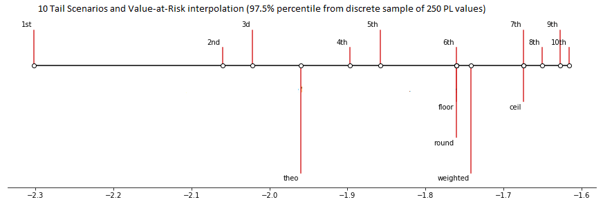
Consider the following example. This is a plot of the 10 smallest values in a sample of 250 values drawn from the standard normal distribution. The plot shows the theoretical 2.5% quantile of the standard normal distribution (“theo”) as well as various types of 97.5 percentile estimation (floor, ceil, weighted, etc).

Atoti Market Risk supports multiple types of VaR estimation, as described in this chapter.
Calculation steps
The algorithm can be described as follows:
- Compute quantile as (1-confidence level)
- Compute adjacent ranks based on the value of the level
[Quantiles].[Quantiles].[QuantileName], quantile and discrete sample size - Sort PL and obtain PL values for the adjacent ranks
and approximate VaR from the PL values using the interpolation formula controlled by the value of the level
[Rounding].[RoundingMethods].[MethodName]
Computing adjacent ranks
The value of the level [Quantiles].[Quantiles].[QuantileName] is used to determine the rank calculation:
| Member value | Description | Formula for rank | Example | Notes |
|---|---|---|---|---|
| Centered | Corresponds to the “First variant, C=1/2” of the interpolation variants described on this wiki | $x = quantile * vectorSize + 0.5$ | (1-97.5%) x 250 + 0.5 = 6.75 | |
| Equal Weight | Corresponds to the “Third variant, C=0” of the interpolation variants described on this wiki | $x = quantile * (vectorSize+1)$ | (1-97.5%)x (250+1) = 6.275 | default option |
| Exclusive | $x = quantile * (vectorSize+1)-1$ | (1-97.5%)x (250+1)-1 = 5.275 | ||
| Simple | $x = quantile * vectorSize$ | (1-97.5%)x 250 = 6.25 |
Based on the computed rank $x$, we can obtain various adjacent ranks:
- $x_{lower}$ = $round_{down}(x)$
- $x_{higher}$ = $round_{up}(x)$
- $x_{nearest}$ = $round(x)$
- $x_{nearestEven}$ = $round_{toEven}(x)$
- $weight$ = $fractionalPart(x)$
and the corresponding P&L values (in the sorted P&L vector):
- $PL_{lower}$ as the value of the sorted P&L vector at rank $x_{lower}$
- $PL_{higher}$ as the value of the sorted P&L vector at rank $x_{higher}$
- $PL_{nearest}$ as the value of the sorted P&L vector at rank $x_{nearest}$
- $PL_{nearestEven}$ as the value of the sorted P&L vector at rank $x_{nearestEven}$
VaR approximation
The value of the level [Rounding].[RoundingMethods].[MethodName] is be used to control the interpolation.
| Property value | Description | Formula for VaR | Example | Notes |
|---|---|---|---|---|
| Floor | Simulated PL for the lower of the adjacent ranks | VaR = $PL_{lower}$ | For $x$ = 6.25, the PL value at rank 6 is taken as the VaR. | |
| Ceil | Simulated PL for the higher of the adjacent ranks | VaR = $PL_{higher}$ | For $x$ = 6.25, the PL value at rank 7 is taken as the VaR. | default option |
| Weighted | Simulated PL linearly interpolated between the adjacent ranks | VaR = $weight * PL_{lower} + (1-weight) * PL_{higher}$ | For $x$ = 6.25, the linear interpolation beween PL value at rank 6 and PL value at rank 7 at the point $x$ = 6.25 is taken as the VaR. | |
| Round | Simulated PL for the nearest rank | VaR = $PL_{nearest}$ | For $x$ = 6.25, the PL value at rank 6 is taken as the VaR. | |
| For $x$ = 6.75, the PL value at rank 7 is taken as the VaR. | ||||
| For $x$ = 7.5, the PL value at rank 8 is taken as the VaR. | ||||
| For $x$ = 8.5, the PL value at rank 9 is taken as the VaR. | ||||
| For $x$ = 9.5, the PL value at rank 10 is taken as the VaR. | ||||
| Round Even | Simulated PL for the nearest rank with rounding half to even | VaR = $PL_{nearestEven}$ | For $x$ = 6.25, the PL value at rank 6 is taken as the VaR. | |
| For $x$ = 6.75, the PL value at rank 7 is taken as the VaR. | ||||
| For $x$ = 7.5, the PL value at rank 8 is taken as the VaR. | ||||
| For $x$ = 8.5, the PL value at rank 9 is taken as the VaR. | ||||
| For $x$ = 9.5, the PL value at rank 10 is taken as the VaR. |