ActivePivot Concepts in a Nutshell

Online analytical processing (OLAP) is about getting as much useful information as possible out of business data while this data is rapidly and continuously changing. It lets its users structure the business data into multi-dimensional cubes from which they can subsequently extract valuable insights, by means of sophisticated summaries and selective drill-downs.

ActivePivot represents a robust and powerful in-memory OLAP solution designed to provide a unique combination of analysis depth, flexibility and real-time performance. Its real-time push technology can aggregate multiple sources of data simultaneously, enabling timely decision making, fast navigation and slice and dice filtering. ActivePivot also allows queries to run continuously, and can generate real-time alerts on Key Performance Indicators (KPIs). This, combined with the in-memory computing paradigm, enables the performing of real-time analytics involving complex business logic.

Data Loading Flow in an ActivePivot Project

The data, coming from one or several sources, is enriched and stored in the datastore. The datastore is relational. Each record in the base store is called a fact. The facts can be enriched with data from other stores, linked through references. Each fact is published to the ActivePivot cube, along with its referenced data, in a single denormalized fact record. The fact is then aggregated into the cube, the level of detail retained being defined by the cube configuration.

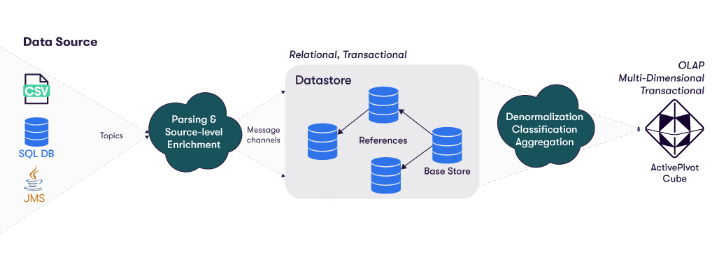
To better understand how to load data into the datastore, you can have a look at the Data Sources Introduction and Datastore overview.

Defining the Cube

To define a cube:

1. Select the fields from the datastore that are to be used in the cube. The selection starts from a base store and can add fields from its referenced stores.
2. Tag each field as a Classifier (C) or a Measure (M).
3. Specify cube axes based on the Classifier fields.
4. Specify aggregations on the Measure fields. If the cube materializes its aggregations in a BITMAP, those aggregations are computed at transaction time. Otherwise, they are computed at query time (cube configured as JUST IN TIME (JIT)).
5. Specify post-processors to be evaluated from other measures. The post-processors can be evaluated from aggregated measures, other post-processors, or a mix of both. The post-processed measures are always evaluated at query time, even when the "simple" aggregations are materialized in a BITMAP.

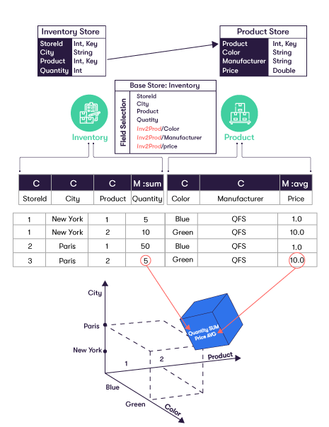
Every record in the base store is published as a single fact into the cube. Each fact is denormalized according to the field selection specified. Each fact is classified based on the values specified for each field tagged as a Classifier (C). Each classified value contributes members to its corresponding axes in the cube. For example, the City axis has the members Paris and New York. The measures in each fact are aggregated at the location specified by its classification (axis values). Aggregation is performed using the function specified (sum, avg, min, etc.)

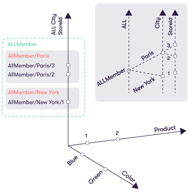
Each cube axis is defined by a hierarchy, which can be composed of nested levels of classified fields (C). By default, each cube axis has a top level classifier of ALL, which corresponds to the aggregation of all its nested members. In our example, we can define a nested hierarchy of City and StoreId. This is a natural hierarchy because the set of stores for any given city does not overlap with the set of stores for a different city. With the ALL top level classifier, the axis would look like:

ActivePivot Cube Locations

A cube location specifies coordinates on each axis of the cube.

• A point location specifies a single distinct coordinate on each axis. Note that the axis coordinate can be a top level entry, which represents the aggregation of its children.
• A range location specifies a set of coordinates on at least one axis. A range location represents a set of point locations. A wildcard coordinate (noted as a star: *) can be used to represent the set of all children at the given classification level.

Cube measures (aggregates or post-processors) are referenced by their location in the cube:

• A point location will reference the measure to a specific coordinate
• A range location will reference the measures for each point location the range location represents.

Here are some examples :

• The cube facts

  C StoreId	C City	C Product	M:sum Quantity	C Color	C Manufacturer	M:avg Price
  1	New York	1	5	Blue	AV	1.0
  1	New York	2	10	Green	AV	10.0
  2	Paris	1	50	Blue	AV	1.0
  2	Paris	2	20	Green	AV	10.0
  3	Paris	1	10	Blue	AV	1.0
  3	Paris	2	5	Green	AV	10.0

• The cube axis

  Axis Name	Classifiers
  Stores	ALL City StoreId
  Products	ALL Product
  Colors	ALL Color
  Manufacturers	ALL Manufacturer

• Some point locations

  Axis value given in the location				Measure value for the given location
  Stores	Product	Color	Manufacturer	Quantity.SUM	Price.AVG
  Green product 2 manufactured by AV in store 3
  AllMember/Paris/3	AllMember/2	AllMember/Green	AllMember/AV	5	10.0
  Green product 2 manufactured by AV in Paris (e.g. aggregation of stores 2 and 3)
  AllMember/Paris	AllMember/2	AllMember/Green	AllMember/AV	25	10.0
  Total (everything)
  AllMember	AllMember	AllMember	AllMember	100	5.5

• Some range locations

  Axis value given in the location				Measure value for the given location
  Stores	Products	Colors	Manufacturers	Quantity.SUM	Price.AVG
  Green product 1 manufactured by AV in store 3, and green product 2 manufactured by AV in store 3
  AllMember/Paris/3	AllMember/[1,2]	AllMember/Green	AllMember/AV	Product 1: null Product 2: 5	Product 1: null Product 2: 10.0
  Each product color manufactured by AV in Paris
  AllMember/Paris	AllMember	AllMember/*	AllMember/AV	Color Blue: 60 Color Green: 25	Color Blue: 1.0 Color Green: 10.0

Custom Measures in ActivePivot

Custom measures are evaluated at query time based on other measures in the cube. They can either be created by extending abstract post-processor classes provided in the product, or by using Copper to easily write the computations to be performed while abstracting from the post-processors framework.

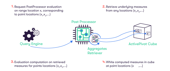
The evaluation method of a post processor is called with a point or range location and is provided an AggregatesRetriever object, which can look up other measures in the cube at any location.

The measures that a post-processor needs in order to compute its result are called underlying measures. The act of retrieving the underlying measures before the computation of the post-processor measure is called prefetching. Prefetchers are defined in the post-processor and are resolved at query planning time: it allows for the prefetched measures to be planned efficiently and eventually shared amongst several post-processors. Prefetching is important for query performance. When the AggregatesRetriever is asked for a measure/location that was not prefetched, its behavior depends on the IMissedPrefetchBehavior context value (default behavior is retrieving the value after logging a warning).

The AggregatesRetriever object is used as an input/output for the measures. It is used to retrieve the prefetched measures, but also to write the result of the post processor evaluation into the cube at point locations. The retriever can only write results at point locations belonging to the original range location passed into the evaluation method.

There is a whole typology of computational logic provided with the product.

The simplest computations are performed by a basic post-processor: underlying measures are all retrieved for the exact same location at which the post-processor results are written.

Another very useful logic in ActivePivot projects is the dynamic aggregation: underlying measures are retrieved at a specific level on each axis that can be more detailed than the aggregation level of the post-processor result. The level at which the underlying measures are retrieved is called the leaf level of the dynamic aggregation post-processor. The post-processor does its computations at leaf level, then aggregates the results to give its result at the requested level.

Note that if the requested level is more detailed than the leaf level, there is no aggregation to perform and the dynamic aggregation post-processor behaves like a basic post-processor.

Here is an example :

• The cube aggregated measures:

  Stores	Products	Colors	Manufacturers	Quantity.SUM	Price.AVG
  AllMember	AllMember/1	AllMember	AllMember	65	1.0
  AllMember	AllMember/2	AllMember	AllMember	35	10.0
  AllMember	AllMember	AllMember	AllMember	100	5.5

• A basic post-processor that computes the cost by multiplying the quantity by the price would compute the cost as this:

  Stores	Products	Colors	Manufacturers	Quantity.SUM	Price.AVG	BasicCost
  AllMember	AllMember/1	AllMember	AllMember	65	1.0	65.0
  AllMember	AllMember/2	AllMember	AllMember	35	10.0	350.0
  AllMember	AllMember	AllMember	AllMember	100	5.5	550.0

• A dynamic aggregation post-processor that goes down to Product level, then multiplies the quantity by the price and aggregates by sum, would compute the cost as this:

  Stores	Products	Colors	Manufacturers	Quantity.SUM	Price.AVG	DynAgCost
  AllMember	AllMember/1	AllMember	AllMember	65	1.0	65.0
  AllMember	AllMember/2	AllMember	AllMember	35	10.0	350.0
  AllMember	AllMember	AllMember	AllMember	not retrieved	not retrieved	415.0

Note that the grand total is not the same when we use the basic post-processor and when we use the dynamic aggregation post-processor, while the results at product level are the same. If we were to only ask for the grand total, the basic post-processor would only retrieve the underlying measures at grand total level, while the dynamic aggregation post-processor would need the underlying measures for both Product 1 and Product 2.

Is the cube only a logical construct ?

The ActivePivot Cube is a conceptual view of the data stored in the datastore. Not all constituents of the cube are actually materialized in memory on a long-term basis.

• The hierarchies are materialized and updated at each transaction. We recommend using as hierarchies only the fields that are actually used to slice and dice the data, not all the non numerical fields of the datastore. We especially recommend avoiding high cardinality hierarchies when possible.

• The custom measures (also known as post-processed measures) are not materialized: since those measures are computed from Java code, their value can be impacted by other events than the transactions, and they are only computed when a query needs them

• The "simple" aggregations (direct aggregations from measures present in the datastore, defined only by the underlying field and an aggregation function plugin key, such as SUM, AVG, MIN...) can be materialized or not depending on the Aggregates Provider implementation.

  • For the Just in Time provider (JIT), no aggregation is materialized and everything is computed at query time.
  • For the other providers, the aggregations are materialized at the lowest level of detail configured for the provider. For example, geographical data can be available in the datastore at the address level, but be aggregated in a LEAF provider at the city level. A query at the state level will be aggregated at query time from the LEAF provider, not from the datastore, thus providing greater query performance (at the cost of memory consumption to maintain the LEAF aggregated data).
  • It is possible to mix several providers in order to get the appropriate trade-off between memory consumption and query performance: a JIT provider for the lowest detail level, then one or even several other providers for the most-often queried aggregation levels. These providers are then called "partial" providers. Partial providers can also choose the measures that are materialized. The appropriate way to retrieve an aggregate will be decided at query time depending on the query measures and locations.

A cube allows viewing data from different points of view by selecting which dimensions to analyse and which measures to view. However, if there are different use cases in which the data are analysed in specific ways, it is possible to define several cubes on the same datastore.