Component Measures
Contributory measures are used by Risk Managers to analyze the impact of a Sub-Portfolio on the Value at Risk of the total Portfolio. These measures can help to track down individual trades that have significant effects on VaR. Furthermore, contributory measures can be a useful tool in hypothetical analyses of portfolio development versus VaR development.
Basic Usage
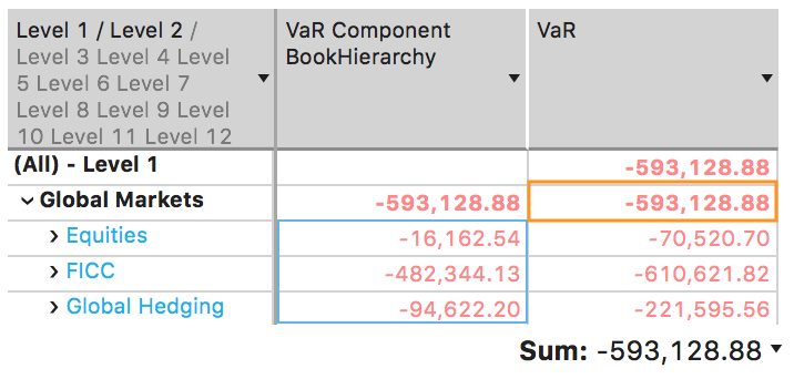
In the below screenshot you can see a pivot table, displaying VaR and VaR Component BookHierarchy. The total of the Component VaR for the sub portfolios under the “Global Markets” node is equal to the VaR value computed for the “Global Markets”.
Component VaR (CoVaR)
Definition
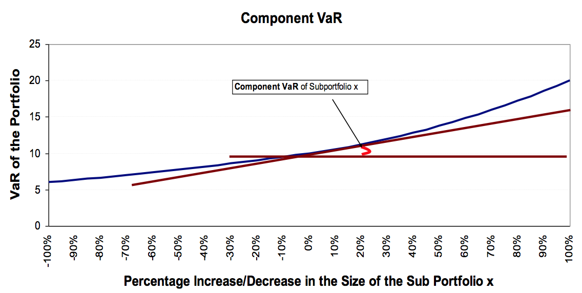
The Component VaR of Sub-Portfolio x measures the rate of change of the VaR of Portfolio X with respect to an incremental change in the size of Sub-Portfolio x.
$$CoVaR_x=\frac{\partial VaR(X)}{\partial w_x}$$
where $w_x$ is the weight of Sub- Portfolio x in Portfolio X.
Component VaR is a very useful tool to examine the overall impact of local changes in a Sub-Portfolio upon the total Portfolio. It is an additive measure so that the Component VaRs of all Sub-Portfolios add up to the VaR of the total Portfolio.
In the Figure below, the CoVaR equals to the slope of the tangent line at point ($VaR_{wx}$, $w_x+0% \cdot w_x$).
Calculation Method
For a parent portfolio $X$ with $N$ components $Y_1$, $Y_2$, …, $Y_N$ the algorithm1 to compute CoVaRs is:
Regress:
$$Y=a+b \cdot X + c \cdot X^2$$
Calculate:
$$A=\begin{pmatrix} L & \sum x & \sum x^2 \\\ \sum x & \sum x^2 & \sum x^3 \\\ \sum x^2 & \sum x^3 & \sum x^4 \end{pmatrix}\rightarrow A^{-1}$$
$A^{-1}$ - getting the inverse matrix.
Start Loop: For i = 1 to N:
- Calculate:
$$B_i=\begin{pmatrix} \sum y_i\\\ \sum xy_i\\\ \sum y_ix^2 \end{pmatrix}$$
- Multiply:
$$A^{-1} \cdot B_i=\begin{pmatrix} a\\\ b\\\ c \end{pmatrix}$$
to get a, b, c the parameters of the regression.
- Compute:
$$CoVaR_i = -\left [ a+b \cdot(-VaR) +c \cdot VaR^2 \right ]$$
- Compute:
$$CoVaR_i^{percentage} = \frac{-\left [ a+b \cdot(-VaR) +c \cdot VaR^2 \right ]}{VaR}$$
End Loop: Next i
All sums, within matrices A and B, span for “ranked” vector scenario ids starting from 1 up to L, with 1 the most negative PnL value for the parent portfolio.
For example:
$$\sum_{j}x^2=x_1^2+x_2^2+…+x_L^2$$
$$\sum_{j}xy_i=x_1y_{i1}+x_2y_{i2}+…+x_Ly_{iL}$$
where $$x_j$$ is the jth PnL of the “ranked” parent portfolio scenario ids and $$y_{ij}$$ is its ith component’s PnL value on jth scenario id.
$L$ denotes the number of scenario ids included in the regression.
Delta Component VaR (Delta CoVaR )
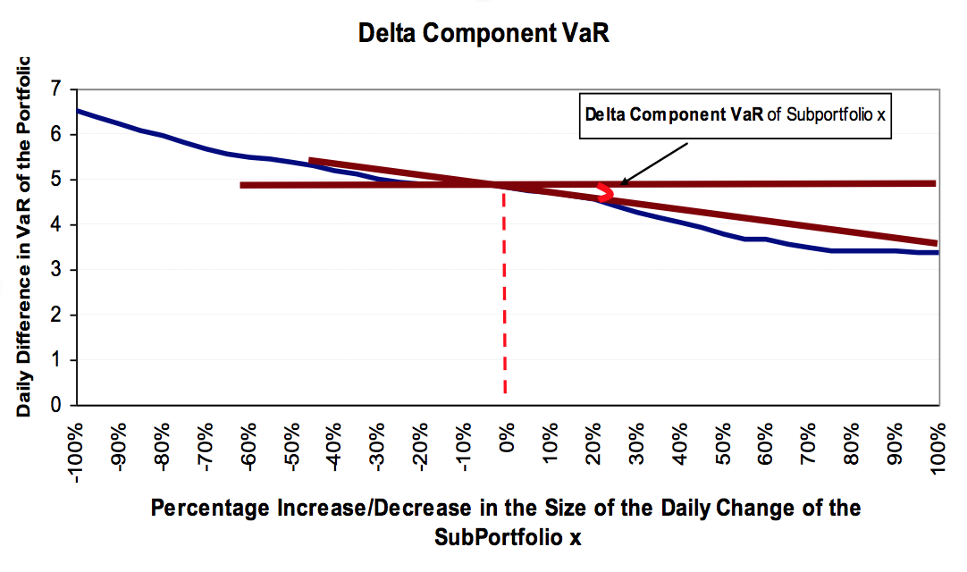
The Delta Component VaR of Sub-Portfolio x measures the rate of change of a Portfolio’s daily change in VaR (Delta VaR(X)) with respect to an incremental change in a Sub-Portfolio’s daily change in size (Delta wx).
The Delta Component VaR is a very useful tool to examine the overall impact of local changes in a Sub-Portfolio upon the total Portfolio’s daily changes in VaR. Delta Component VaR is an additive measure so that the Delta Component VaRs of all Sub Portfolios add up to the daily change in VaR of the total Portfolio.
$$DeltaCoVaR_x=\frac{\partial \left ( \Delta VaR(X) \right )}{\partial \left (\Delta w_x \right )}$$
In the Figure below, CoVaR equals to the slope of the tangent line at point (ΔVaR, Δwx+0% * Δwx).
Calculation Method
Delta Component VaR or Delta CoVaR will be computed in the same fashion as the CoVaR by using the quadratic regression technique.
For a parent portfolio $X$ with $N$ components $Y_1$, $Y_2$, …, $Y_N$ the algorithm1 to compute DeltaCoVaRs is:
Calculate:
$$A=\begin{pmatrix} L & \sum \Delta x & \sum \Delta x^2 \\\ \sum \Delta x & \sum \Delta x^2 & \sum \Delta x^3 \\\ \sum \Delta x^2 & \sum \Delta x^3 & \sum \Delta x^4 \end{pmatrix}\rightarrow A^{-1}$$
$A^{-1}$ - getting the inverse matrix.
Start Loop: For i = 1 to N;
- Calculate:
$$B_i=\begin{pmatrix} \sum \Delta y_i\\\ \sum \Delta x \Delta y_i\\\ \sum \Delta y_i \Delta x^2 \end{pmatrix}$$
- Multiply:
$$A^{-1} \cdot B_i=\begin{pmatrix} a\\\ b\\\ c \end{pmatrix}$$
to get a, b, c the parameters of the regression.
- Compute:
$$\Delta CoVaR_i = -\left [ a+b \cdot(-\Delta VaR) +c \cdot \Delta VaR^2 \right ]$$
- Compute:
$$\Delta CoVaR_i^{percentage} = \frac{-\left [ a+b \cdot(-\Delta VaR) +c \cdot \Delta VaR^2 \right ]}{\Delta VaR}$$
End Loop: Next i
The PnL vector inputs for the parent portfolio $X$ with $N$ components $Y_1$, $Y_2$, …, $Y_N$ are now equal to the daily PnL changes from one business date to the next business date.
The changes of the parent portfolio are related to the changes to its N components with the following equations:
$$x_i^{cob}-x_i^{cob-1}=\left ( y_1i^{cob} - y_1i^{cob-1} \right )+\left ( y_2i^{cob} - y_2i^{cob-1} \right )+…+\left ( y_Ni^{cob} - y_Ni^{cob-1} \right ), \text{ for i=1 to 500}$$
where $$x_i$$ is the most backdated PnL date at cob for parent portfolio X.
All sums, within matrices A and B, span for “ranked” vector scenario ids starting from 1 up to L, with 1 the most negative PnL value for the parent portfolio.
For example, $$\sum_{j} \Delta x^2=\Delta x_1^2+\Delta x_2^2+…+\Delta x_L^2$$ and $$\sum_{j}\Delta x\Delta y_i=\Delta x_1 \Delta y_{i1}+\Delta x_2 \Delta y_{i2}+…+\Delta x_L \Delta y_{iL}$$, where $$\Delta x_j$$ is the daily change of the jth PnL of the “ranked” parent portfolio scenario ids and $$\Delta y_{ij}$$ its ith component’s PnL value on jth scenario id.
$\Delta VaR$ is the change in VaR of the parent node from cob to cob-1.
$L$ denotes the number of scenario ids included in the regression.
Algebraic solution
Here is the algebraic solution for the a, b, c.
$$a=\frac{\sum y\sum x^2-\sum xy\sum x+c\sum x^3\sum x-c\left ( \sum x^2 \right )^2}{n\sum x^2-\left ( \sum x \right )^2}$$
$$b=\frac{n\sum{xy}-nc\sum{x^3}+c\sum{x^2}\sum{x}-\sum{y}\sum{x}}{n\sum x^2-\left ( \sum x \right )^2}$$
$$c=\frac{\left ( \sum{x^2y} \right )\left ( n\sum{x^2}-\left ( \sum{x} \right )^2 \right )-\left ( \sum{x^2} \right )^2\sum{y}+\sum{xy}\sum{x}\sum{x^2}}{2\sum{x^3}\sum{x}\sum{x^2}-\left ( \sum{x^2} \right )^3-n\left ( \sum{x^3}\right )^2+\sum{x^4\left ( n\sum{x^2}-\left ( \sum{x} \right )^2 \right )}}\\+\frac{-n\sum{x^3}\sum{xy}+\sum{y}\sum{x}\sum{x^3}}{2\sum{x^3}\sum{x}\sum{x^2}-\left ( \sum{x^2} \right )^3-n\left ( \sum{x^3}\right )^2+\sum{x^4\left ( n\sum{x^2}-\left ( \sum{x} \right )^2 \right )}}$$
-
The regression parameters a, b, c can also be computed algebraically. See Algebraic solution. ↩︎ ↩︎