Taylor VaR
Overview
With the sensitivities it is possible to compute an approximated PnL of a product using the Taylor formula.
$${\displaystyle f(a+shift)=f(a)+\nabla f(a)\cdot shift+{\frac {1}{2}}shift^{T}\mathbb {H}_f(a)shift+\mathcal{O}(shift^2)}$$
In this formula:
- $a$ is the current market state.
- $shift$ is a market shift, it is a vector kind value as multiple market data can be shifted for the same scenario.
- $\nabla f(a)$ is the gradient of $f$ at $a$, it’s a vector of the first-order risk factors such as delta, vega or correlation.
- $\mathbb {H}_f(a)$ is the Hessian matrix of $f$ at $a$, it’s a matrix containing the second-order risk factors such as gamma, cross-gamma, vanna or volga.
On an expanded scalar view we can write down the formula as: $$f(a+shift) = f(a) + \sum_{i=1}^n \frac{\partial f}{\partial x_i}(a) \cdot shift_i + \frac{1}{2} \sum_{i=1}^n \sum_{j=1}^n \frac{\partial^2 f}{\partial x_i \partial x_j}(a)\cdot shift_i \cdot shift_j+\mathcal{O}(shift^2)$$
This formula is applied for each scenario to obtain a PnL vector with one entry per scenario.
Cube process
In the cube, the PnL computation with the Taylor formula is not performed per trade, but instead per risk factor, by applying the Taylor part of the formula to this specific risk factor / market shift pair.
The applied formula is the same as the one used for the PnL Explain functionality.
As the next stage of the formula is purely linear, with the help of cube aggregation, we can output PnL per trade, risk factor, and so on.
The market shift is provided directly as a vector compatible with the VaR scenarios.
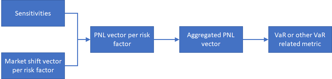
So to be clear we will compute the PnL per scenario for each Sensitivity Kind x Risk Factor. The result will be aggregated by Sensitivity Kind and then consolidate on a global PnL vector.
$$PnL_{scenario}=f(a+shift_{scenario})-f(a)=\sum_{i=1}^n \frac{\partial f}{\partial x_i}(a) \cdot shift_{i,scenario} + \frac{1}{2} \sum_{i=1}^n \sum_{j=1}^n \frac{\partial^2 f}{\partial x_i \partial x_j}(a)\cdot shift_{i,scenario} \cdot shift_{j,scenario}$$
Please note that $$ \frac{1}{2} \sum_{i=1}^n \sum_{j=1}^n \frac{\partial^2 f}{\partial x_i \partial x_j}(a)\cdot shift_{i,scenario} \cdot shift_{j,scenario}= \frac{1}{2}\sum_{i=1}^n \frac{\partial^2 f}{\partial x_i^2 }(a)\cdot shift_{i,scenario}^2+\sum_{i=1}^n \sum_{j>i}^n \frac{\partial^2 f}{\partial x_i \partial x_j}(a)\cdot shift_{i,scenario} \cdot shift_{j,scenario}$$
- The $\frac{1}{2}\sum_{i=1}^n \frac{\partial^2 f}{\partial x_i^2 }(a)\cdot shift_{i,scenario}^2$ part is handled by the “One risk factor” computation.
- The $\sum_{i=1}^n \sum_{j>i}^n \frac{\partial^2 f}{\partial x_i \partial x_j}(a)\cdot shift_{i,scenario} \cdot shift_{j,scenario}$ part is handled by the “Two risk factors” computation. The $j>i$ replaces the $\frac{1}{2}$ in the formula.
We regroup the computation by risk factor or pair of risk factor for cross-gamma and vanna, and use one PnL formula the sensitivity kind x risk class.
$$PnL_{scenario}=\sum_{riskFactor} PnL_{riskFactor}(shift_{riskFactor,scenario})+\sum_{riskFactor1,riskFactor2} PnL_{riskFactor1,riskFactor2}(shift_{riskFactor1,scenario},shift_{riskFactor2,scenario})$$
Computation
One risk factor
The $PnL_{riskFactor}(shift_{riskFactor,scenario})$ is computed by the ScalarPnlVectorFromRiskSensiPostProcessor post-processor.
The formula is provided by the spring bean of type ITaylorVarFormulaProvider, with the function
DoubleBinaryOperator getTaylorVarFormula(ConcurrentMap<Object, Object> cache, String sensitivityKind, String sensitivityName, String riskClass);
It uses as parameters:
cache: The query cache.sensitivityKind: The formal name of the current metric chain.sensitivityName: The name of the sensitivity coming from the TradeSensitivities store.riskClass: The risk class coming from the TradeSensitivities store.
It returns a function $PnL(sensitivity, shift_{riskFactor,scenario})$. The following functions can be provided:
| type | Formula |
|---|---|
| Absolute / Relative / DHS | $$PnL(sensitivity, shift)=sensitivity \cdot \frac{(shift \cdot priceFactor)^{derivativeOrder}}{derivativeOrder!}$$ |
| FXRelative | $$PnL(sensitivity, shift)=sensitivity \cdot \frac{\left(\left(1-\frac{1}{1+shift} \right)\cdot priceFactor\right)^{derivativeOrder}}{derivativeOrder!}$$ |
The type, derivative-order, price-factor are configured by the properties.
To find the right property set, we will look for the following path:
mr.sensi.rules.sensitivityName.taylor-var.riskClassmr.sensi.rules.sensitivityKind.taylor-var.riskClassmr.sensi.rules.sensitivityName.pnl-explain.riskClassmr.sensi.rules.sensitivityKind.pnl-explain.riskClass
In case of the use of a Ladder, the sensitivity is computed from the Ladder and the shift (see Sensitivity ladders), before applying the PnL formula.
Two risk factors
The $PnL_{riskFactor1,riskFactor2}(shift_{riskFactor1,scenario},shift_{riskFactor2,scenario})$ is computed by the ScalarPnlVectorFromCrossRiskSensiPostProcessor post-processor.
We will grab two formula from the spring bean of type ITaylorVarFormulaProvider.
The first axis has the name sensitivityKind1, for example “cross-gamma1”, used as the sensitivityKind to grab the formula.
The second axis has the name sensitivityKind2, for example “cross-gamma2”, used as the sensitivityKind to grab the formula.
The two formula will be applied one after the other.
$$PnL(shift_{riskFactor1},shift_{riskFactor2}) =PnL_2(PnL_1(sensitivity, shift_{riskFactor1}), shift_{riskFactor2})$$
In case of the use of a Ladder, the sensitivity is computed from the Ladder and the shift of the first axis (see Sensitivity ladders), before applying the PnL formula on both.
Sources
The risk factor values are read straight from the aggregated sensitivity metrics. The market shifts are loaded directly from the MarketShifts store.
Limitations
The market shifts must be the same kind as the sensitivity, that is, either absolute or relative.