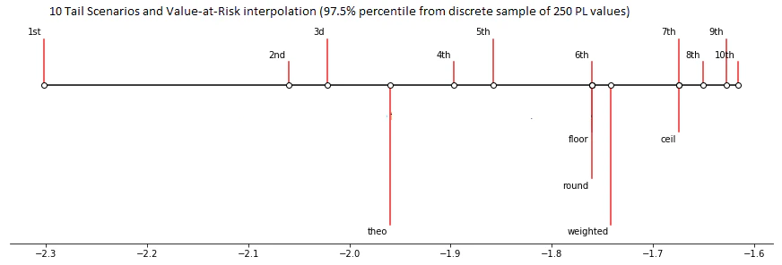
 Atoti Market Risk supports multiple types of VaR estimation, as described in this chapter.
## Calculation steps
The algorithm can be described as follows:
* Compute quantile as (1-confidence level)
* Compute adjacent ranks based on the value of the level `[Quantiles].[Quantiles].[QuantileName]`, quantile and discrete sample size
* Sort PL and obtain PL values for the adjacent ranks
and approximate VaR from the PL values using the interpolation formula controlled by the value of the level `[Rounding].[RoundingMethods].[MethodName]`
## Computing adjacent ranks
The value of the level `[Quantiles].[Quantiles].[QuantileName]` is used to determine the rank calculation:
Atoti Market Risk supports multiple types of VaR estimation, as described in this chapter.
## Calculation steps
The algorithm can be described as follows:
* Compute quantile as (1-confidence level)
* Compute adjacent ranks based on the value of the level `[Quantiles].[Quantiles].[QuantileName]`, quantile and discrete sample size
* Sort PL and obtain PL values for the adjacent ranks
and approximate VaR from the PL values using the interpolation formula controlled by the value of the level `[Rounding].[RoundingMethods].[MethodName]`
## Computing adjacent ranks
The value of the level `[Quantiles].[Quantiles].[QuantileName]` is used to determine the rank calculation:
| Member value | Description | Formula for rank | Example | Notes |
|---|---|---|---|---|
| Centered | Corresponds to the “First variant, C=1/2” of the interpolation variants described on this wiki | $x = quantile * vectorSize + 0.5$ | (1-97.5%) x 250 + 0.5 = 6.75 | |
| Equal Weight | Corresponds to the “Third variant, C=0” of the interpolation variants described on this wiki | $x = quantile * (vectorSize+1)$ | (1-97.5%)x (250+1) = 6.275 | default option |
| Exclusive | $x = quantile * (vectorSize+1)-1$ | (1-97.5%)x (250+1)-1 = 5.275 | ||
| Simple | $x = quantile * vectorSize$ | (1-97.5%)x 250 = 6.25 |
| Property value | Description | Formula for VaR | Example | Notes |
|---|---|---|---|---|
| Floor | Simulated PL for the lower of the adjacent ranks | VaR = $PL_{lower}$ | For $x$ = 6.25, the PL value at rank 6 is taken as the VaR. | |
| Ceil | Simulated PL for the higher of the adjacent ranks | VaR = $PL_{higher}$ | For $x$ = 6.25, the PL value at rank 7 is taken as the VaR. | default option |
| Weighted | Simulated PL linearly interpolated between the adjacent ranks | VaR = $weight * PL_{lower} + (1-weight) * PL_{higher}$ | For $x$ = 6.25, the linear interpolation beween PL value at rank 6 and PL value at rank 7 at the point $x$ = 6.25 is taken as the VaR. | |
| Round | Simulated PL for the nearest rank | VaR = $PL_{nearest}$ | For $x$ = 6.25, the PL value at rank 6 is taken as the VaR. | |
| For $x$ = 6.75, the PL value at rank 7 is taken as the VaR. | ||||
| For $x$ = 7.5, the PL value at rank 8 is taken as the VaR. | ||||
| For $x$ = 8.5, the PL value at rank 9 is taken as the VaR. | ||||
| For $x$ = 9.5, the PL value at rank 10 is taken as the VaR. | ||||
| Round Even | Simulated PL for the nearest rank with rounding half to even | VaR = $PL_{nearestEven}$ | For $x$ = 6.25, the PL value at rank 6 is taken as the VaR. | |
| For $x$ = 6.75, the PL value at rank 7 is taken as the VaR. | ||||
| For $x$ = 7.5, the PL value at rank 8 is taken as the VaR. | ||||
| For $x$ = 8.5, the PL value at rank 9 is taken as the VaR. | ||||
| For $x$ = 9.5, the PL value at rank 10 is taken as the VaR. |