Partitioning and NUMA awareness in Atoti
Data partitioning represents an important concept in Atoti, and understanding it is crucial in bringing performance to a project. It is:
- An enabler of true multi-core scalability
- An accelerator of data loading and querying
- The foundation for Atoti's NUMA awareness
Partitioning 101
Defining a partitioning on a store in Atoti consists of clustering the data that this store holds, separating records into different partitions. It is done on a per-store basis, and is optional (but strongly recommended on stores of importance).
Choices made for partitioning drastically influence the performance of the datastore, because all operations in a partition are single-threaded.
Here are two examples of poor partitioning choices:
- Disproportionate partitions: if one partition holds 10 times as many records as the others, all partitions will wait on this particular partition to finish an operation that equally hits all partitions. This mistake can be observed with tools like JConsole during the data loading, for instance. As the CPU's % usage curve will, for a short time, be close to 100% usage, before falling quickly to single-digit percentages while only the remaining partition loads data.
- Having too many partitions: if a store has a partition count an order of magnitude higher than the CPU count of the server running the application, query performance will be hit by context switching.
Once the configuration is applied, partitioning works transparently for both users and developers: Partitions are an internal concept, and both records and queries are automatically dispatched to the appropriate partitions.
Fields choice and strategy
Typically, a partitioning field is chosen first, and then a strategy is picked. These must ensure two goals are achieved:
An even distribution of records across the partitions. This allows the work performed by the processing cores to be distributed efficiently for both loading and querying.
An appropriate partitioning strategy choice. An application that requires intensive data maintenance operations such as "drop all of last week's records" may find it extremely efficient to have the records in different partitions based on a key field related to the date. Indeed, if a partition exactly holds all the records for the specific date that correspond to a
removeWherecondition, the entire partition can be dropped instantly. This allows for efficient house-keeping.By contrast, an application that mostly serves queries that apply to very large data sets may want to maximize the usage of the processing resources for querying. In such a case, it may be preferable to use a random partitioning (yet yielding an even distribution of records across partitions), to spread the queried records across all partitions, and thus across all processing units.
An application that is used by multiple users that each have a specific domain may want to partition its data across this user domain, to minimize cross domain data movement and resource sharing.
It is highly encouraged to experiment with several partitioning strategies in a test environment, early on in the project's life-cycle, to find the most optimal design.
Partitioning Constraints
The two following constraints should guide partitioning configuration:
- Key fields constraints: If a store has key fields, the partitioning fields must be among these key fields. A store with no key-fields can be partitioned on any of its dictionarized fields.
- Store reference constraints: The partitioning of the target store (i.e. referenced store) must be implied by the partitioning of the owner store (i.e. base store). This implication is detailed in the section regarding the partitioning across references.
NUMA Awareness and Optimization
NUMA Awareness is only available to Linux servers.
Introduction
Modern CPUs operate considerably faster than the main memory they use. Thus, extracting performance from a modern computer has, for a long time, been a question of installing an ever-increasing amount of high-speed cache memory, and developing increasingly sophisticated algorithms to avoid cache misses.
However, these improvements were overwhelmed by the increase in size of applications running on the servers. On a multi-processor server, a system can even starve several processors, because only one can access the computer's memory at a time. This issue is known as contention.
In the following schema is shown the SMP architecture, which is using a single shared system bus to feed all processors:

The Non-Uniform Memory Architecture (NUMA) attempts to address this issue by providing separate memory for each processor or group of processors, thus avoiding the performance hit with contention.

For problems involving spread data, NUMA can improve the performance over a single shared memory bank by a factor roughly estimated to be the number of separate memory banks (in the case of one memory bank per physical processor, the factor would be equal to the number of processors). However, not all the data is confined to a single task, which means that NUMA systems still need to share data across processors and memory banks, which will slow the system down.
The overall speed increase due to NUMA thus depends heavily on the nature of the running tasks.
Installation
On a Linux system, one must first install the numactl package. The command numactl -H prints
the list of nodes configured on the machine, the CPU and memory characteristics for each node, as
well as a distance matrix, provided by the firmware manufacturer, that indicates the latency between
nodes.
The following represents the output of the command numactl -H on a machine with 2 NUMA nodes,
each one of them regrouping 8 of the CPUs.
The nodes are numbered 0 and 1, and the command shows, for each NUMA node, the associated CPUs' ids,
and associated RAM.
In the given distance matrix, 10 is the default value, given to a processor accessing its own memory
bank. Higher values indicate a higher latency (the given values are somewhat proportional to
the worst-case induced latencies). One can get the absolute latency numbers between NUMA nodes using
Intel's Memory Latency Checker.
root: $ numactl -H
available: 2 nodes (0-1)
node 0 cpus: 0 1 2 3 4 5 6 7
node 0 size: 461823 MB
node 0 free: 451389 MB
node 1 cpus: 8 9 10 11 12 13 14 15
node 1 size: 459776 MB
node 1 free: 449678 MB
node distances:
node   0   1
  0:  10  22
  1:  22  10
Usage in Atoti
Two NUMA policies are available on the Datastore: the data can either be bound to a particular node
or remain free.
To pick a policy, use the -Dactiveviam.pool.policy=<String> option.
For the first policy, one thread pool is allocated per NUMA node.
Each thread of the thread pool is bound to a node, and the thread pool is responsible for any memory
allocation on its node. When data is allocated on a node, it is bound to this specific node, and any
read or write operation will be performed by the associated thread pool.
This maximizes data locality, and minimizes latency.
The option to specify is placed, and represents the default option.
For the second policy, only one thread pool is allocated, spanning across the entire system. The
threads are under the responsibility of the OS, and can move between nodes at any given time. Data
can be allocated on any node, and no effort is made to maximize locality.
The option to specify is free.
The total number of threads can be tuned using the -Dactiveviam.pool.size=<Integer> option.
On a machine with 4 nodes, 64 corresponds to 16 threads per node with the placed policy,
and to 64 threads spanning on the entire system with the free policy.
The default total number of threads is equal to the number of processors as returned by
Runtime.getRuntime().availableProcessors().
Optimal Number of Partitions
In general, processors have multiple physical cores, each of them able to run several processes concurrently, thus emulating more logical cores than there are physical ones. Typically, hyper-threading provides two logical cores for each physical core.
Atoti Server's minimum requirement amounts to one partition per physical processor for any NUMA-aware application. See the NUMA Section above. However, many algorithms in Atoti work best when the threads that run concurrently in the system are each working on their own partition, to minimize contention between the threads.
Therefore, Atoti usually recommends configuring a store to have at least one partition per logical core.
Partitioning Functions
To partition a store is to choose a set of fields, and a set of functions to apply to the data within these fields to select a partition for each record.
Partitioning functions always apply on dictionarized values, thus integers. Indeed, partitioning fields are ensured to be dictionarized.
Value Partitioning
Value Partitioning is a function that assigns one partition per distinct value of the field. In the following example, the store is partitioned on the Date field, each date's trades filling a single partition:
StoreDescription.builder()
    .withStoreName("Trades")
    .withField("Buyer", ILiteralType.STRING)
    .asKeyField()
    .withField("Seller", ILiteralType.STRING)
    .asKeyField()
    .withField("Date", ILiteralType.DATE)
    .asKeyField()
    .withField("Amount", ILiteralType.FLOAT)
    .asKeyField()
    .withValuePartitioningOn("Date");
Pros: Value Partitioning is useful in a system in which house-keeping is important, and deletions happen regularly.
Cons: As the cardinality of the field increases, the number of partitions may become unreasonably large. When choosing this configuration, one must also take into account all the future transactions that might continue adding records (and new partitions) to the system. The distribution of records across partitions can also grow more and more skewed, as it is up to the users to know whether they will be filling the partitions unequally or not.
Modulo Partitioning
Modulo Partitioning on a single field is a function that takes the dictionarized value of the record for
that field, and applies a modulo-N operation to this value to assign a partition to the record.
Thus, a given number of partitions N is decided upon in advance.
A good practice is to select a number of partitions that is a power of 2.
StoreDescription.builder()
    .withStoreName("Trades")
    .withField("TradeId", ILiteralType.INT)
    .asKeyField()
    .withField("Buyer", ILiteralType.STRING)
    .withField("Seller", ILiteralType.STRING)
    .withField("Date", ILiteralType.DATE)
    .withField("Amount", ILiteralType.FLOAT)
    .withModuloPartitioning("TradeId", CPU_COUNT);
Pros: The number of partitions is known in advance. The balancing of the partitions should be near optimal, this is ensured by the use of the dictionarized values, meaning that only existing values are considered. Conversely, if a field only holds the values 1 and 100k, using the raw values might give only one partition containing both values. Using the dictionarized values (1 -> 1, 2 -> 100k) ensures the presence of two partitions.
Cons: The user must make sure there are more distinct values in the partitioning field than there are partitions to ensure that the partitioning is efficient.
A Modulo Partitioning can also be defined on multiple fields. A given number of partitions N is
decided in advance. The partition of a record is determined as follows: an integer value is computed
by a hashing algorithm using the record's dictionarized values on the partitioning fields,
and the modulo function is applied to that result.
StoreDescription.builder()
    .withStoreName("Trades")
    .withField("Buyer", ILiteralType.STRING)
    .asKeyField()
    .withField("Seller", ILiteralType.STRING)
    .asKeyField()
    .withField("Date", ILiteralType.DATE)
    .asKeyField()
    .withField("Amount", ILiteralType.FLOAT)
    .asKeyField()
    .withModuloPartitioning(8, "Buyer", "Date");
Pros: The user keeps control over the amount of partitions while being able to use multiple partitioning fields.
Cons: This function can only be implied by the same type of partitioning, on the same fields, with a compatible modulo function. It can be difficult to use when partitioning across a reference.
There is an API for selecting all key fields, which is
withKeyModuloPartitioning(int).
It is good practice to use a Modulo Partitioning on all key fields as it ensures balanced partitions.
Combining Fields
The datastore allows its users to select a number of store fields and assign a different partitioning function to each field. This is technically called a Cartesian Partitioning.
The partition is determined by combining the results of these functions. As a result of these functions, the set of partitions is the Cartesian Product of the possible results for each partitioning function.
In the following example, assuming the system keeps a week's worth of trades, there are 7 days * 8
possible partitions, which are the Cartesian Product of the possible results for each partitioning
function.
StoreDescription.builder()
    .withStoreName("Trades")
    .withField("Buyer", ILiteralType.STRING)
    .asKeyField()
    .withField("Seller", ILiteralType.STRING)
    .asKeyField()
    .withField("Date", ILiteralType.DATE)
    .asKeyField()
    .withField("Amount", ILiteralType.FLOAT)
    .asKeyField()
    .withValuePartitioningOn("Date")
    .withModuloPartitioning("Seller", CPU_COUNT);
Pros: If a field seems like the obvious choice for a partitioning (like the date for the Trade store), but does not have a high enough cardinality to mobilize the entire CPU, this partitioning function can help attribute records to more partitions, and thus use the CPU more efficiently.
Cons: As the partitioning function gets more complex, it can become harder to ensure that successive transactions will not skew the records' distribution.
Hierarchical Partitioning
Hierarchical Partitioning is another configuration over multiple partitioning fields. It gives more flexibility than the Cartesian Partitioning by giving each partitioning field a separate rule.
An example use case for a Hierarchical Partitioning would be the following: a trading desk is calculating some measures to compare its clients (Buyers). The most trivial partitioning field for this case is the Buyer field, as most queries can be parallelized using this field. However, a small quantity of buyers amount for the vast majority of the trades, which makes the value partitioning a bad configuration.
To keep partitions balanced, the user must add other partitioning fields, like the date, or a modulo over the tradeId. However, a Cartesian Partitioning will over-partition the store, while probably keeping some distribution imbalance (the subsets of partitions corresponding to the big buyers will still hold bigger partitions than the others).
StoreDescription.builder()
    .withStoreName("Trades")
    .withField("Buyer", ILiteralType.STRING)
    .asKeyField()
    .withField("Seller", ILiteralType.STRING)
    .asKeyField()
    .withField("Date", ILiteralType.DATE)
    .asKeyField()
    .withField("Amount", ILiteralType.FLOAT)
    .asKeyField()
    .withPartitioningOn("Buyer")
    .forValues("BigBuyer1", "BigBuyer2")
    // 8 partitions, a multiple modulo partitioning on the key fields, per big buyer
    .useModuloPartitioningOnAvailableKeyFields(CPU_COUNT)
    .forOthers()
    .useSinglePartition();
Pros: Gives full flexibility over the partitioning function, permitting to precisely select the most relevant partitioning.
Cons: As the dataset evolves, the chosen partitioning might lose its relevance and efficiency.
Partitioning across References
In this section, examples of a partitioning across a store reference are presented.
Remember that the partitioning of the target store of a reference must be implied by the partitioning of the owner store, meaning that all records of a partition in the owner store must reference records of the same partition in the target store. Therefore, the partitioning of the target store is a sub-partitioning of the owner store, so there are a lesser or equal number of partitions in the target store than in the owner store.
In the following examples, these notations are used to represent the different partitioning functions:
modulo<N>(<field 1>[, <field 2>, ...])for modulo partitioningvalue(<field>)for value partitioningvalue(A) | value(B) | ...for a partitioning combining multiple functions
Example 1:
Owner store partitioning:
value(A) | modulo8(B) | modulo16(C)
Target store partitioning:value(A) | modulo2(B)This partitioning is valid, as all fields of the target store partitioning are present in the owner store, and
modulo2(B)is a sub-partitioning ofmodulo8(B)because 8 is a multiple of 2. Thus, the partitioning of the target store is implied by the partitioning of the owner store.Here's all other target store partitioning that are valid:
constant,value(A),modulo2(B),modulo4(B),modulo8(B),value(A) | modulo4(B)andvalue(A) | modulo8(B).Example 2:
Owner store partitioning:
modulo8(A) | modulo4(B)
Target store partitioning:value(A) | modulo4(C)This partitioning is invalid for two reasons: field C is a partitioning field in the target store but not in the owner store, and the partitioning function for field A in the target store is not implied by the one for field A in the owner store.
Note that modulo<M>(A) is implied by modulo<N>(A) if and only if N is a multiple of M.
So modulo<N>(A) is always implied by value(A) as value(A) can be seen as a
Modulo-Infinity Partitioning.
Example 3:
Owner store partitioning:
modulo8(A)
Target store partitioning:modulo3(A)This partitioning is invalid because, even if both stores have a Modulo Partitioning on the same field, 3 does not divide 8. Let's see why it would not be compatible: values 0 and 8 belong to the same partition in the owner store; partition 0 (0 % 8 = 0 and 8 % 8 = 0). But these values belong to different partitions in the target store, respectively partitions 0 and 2 (0 % 3 = 0 and 8 % 3 = 2).
Considerations
One must be careful when a partitioning can propagate to another store multiple times. For instance, if an 'Order' store references a 'Customer' store twice, once for the buyer, once for the seller, then the customer store cannot be partitioned without risks of the partitions induced by the two references conflicting.
Partitioning a store referenced by other stores can only be done using fields that belong to the relationship.
Partitioning the base store, which is usually the largest store, is always beneficial.
Aggregate Provider Partitioning
Atoti's Aggregate Providers are also partitioned to provide multithreaded performance at the cube's level.
Both the Bitmap provider and the Leaf provider can be partitioned. The exact same methods and APIs can be used for this purpose.
If no partitioning is defined, Atoti falls back to defining a partitioning for the aggregate providers that closely follows the datastore partitioning.
A user might want to change the partitioning for two major reasons:
- Remedy the limitations encountered when partitioning the base store. If the best field for partitioning is part of a target store referenced from the base store, the latter one might not be optimally partitioned. However, the user can change this with the aggregate providers' partitioning.
- Provide a better partitioning for queries. A partitioning that might be excellent for data loading might not be the best choice for queries that do not require a datastore lookup.
Considerations
One of the main concerns when setting a special partitioning for an Aggregate Provider is the impact it can have on the commit phase, when contributing all the necessary elements of the datastore to the providers, and the hierarchies.
The data must be adapted to be received into the correct provider partition. In some cases, it might be necessary to scan every fact and compute its target partition id to populate the aggregate providers.
However, the true underlying limitation is that operations within a partition are single-threaded. This specifically means that Atoti can only fill a given partition with a single thread. If an aggregate provider partition is being filled by multiple datastore partitions, the changes are queued rather than applied in parallel.
These extra steps may add a cost to commit time and transient memory usage while committing.
Another concern is that when re-partitioning the aggregate provider, one must once again pay attention not to skew the partitions: Let's imagine a well-defined store with a field Date and a field Value, partitioned by Date, and containing:
- (Date: 01/12/20, Value: 1) -> 25M entries
- (Date: 01/12/20, Value: 2) -> 15M entries
- (Date: 02/12/20, Value: 1) -> 27M entries
- (Date: 02/12/20, Value: 2) -> 13M entries
The partitions are balanced within the Datastore, with 40M entries per partition (per Date).
However, let us imagine that we need an Aggregate Provider partitioned by Value. When creating two
partitions, the partition matching the condition Value EQUALS 1 contains 52M entries, while the
one for Value EQUALS 2 contains 28M entries. Thus, there will be some single-threaded work once
partition 2 is filled, but partition 1 is still being fed records.
NUMA Node Selectors
Atoti offers the possibility to define the NUMA node of each partition, whether it is a store partition, or an aggregate provider partition. In an ideal scenario, each connected component should entirely reside within the same NUMA node. For instance, a store partition contributing to an aggregate provider partition should be on the same node as the provider partition, to avoid transferring data from one node to another.
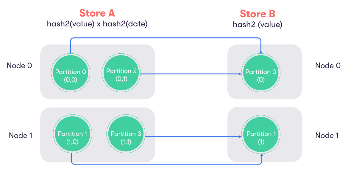
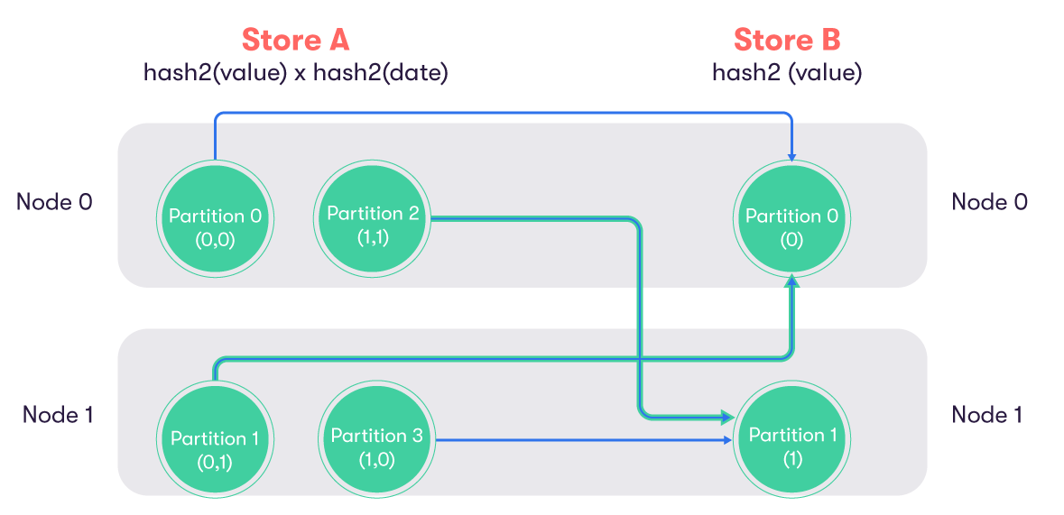
The following example will illustrate the differences between a good and a bad re-partitioning.
Store A and Store B have compatible partitioning:
- Store A :
modulo42(value) | modulo4<2>(date) - Store B :
modulo42(value)The server has 2 NUMA nodes. After applying the modulo transformations, this means that store A can have four different values:(0, 0); (0, 1); (1, 0); (1, 1)as(value, date), while store B can have(0); (1)as(value).
From these combinations, Atoti assigns a unique integer that will become the partition ID. However, these partition IDs do not have a fixed definition, they are attributed as data is inserted in the stores.
For both of the following examples, the first inserted entry for store B has a combination of
(0), and will create the partition 0. Then another entry corresponding to (1) will create
partition 1.
In an ideal scenario, entries will be inserted into store A in the following order:
(0, 0); (1, 0); (0, 1); (1, 1), thus creating the four partitions.
This will result in the following schema, in which all partitions matching the condition
value EQUALS 1 reside on NUMA node 1:

In a less than ideal scenario, entries will be inserted in the store A in the following order:
(0, 0); (0, 1); (1, 1); (1, 0). This results in the following schema, in which data must be
transferred across NUMA nodes:

This happens because the default NUMA selector only uses the partition ID to select the NUMA node, using the modulo function's results, and can be avoided using a custom NUMA selector. Using this selector, the NUMA node is selected solely on the value of the field Value.
StoreDescription.builder()
    .withStoreName("Trades")
    .withField("Date", ILiteralType.DATE)
    .asKeyField()
    .withField("Value", ILiteralType.FLOAT)
    .asKeyField()
    .withModuloPartitioning("Date", 2)
    .withModuloPartitioning("Value", 2)
    .withNumaNodeSelector()
    .withFieldPartitioning("Value");
An aggregate provider partition will be located in the same NUMA node as the Base Store partition that created it. Several Base Store partitions may feed a single aggregate provider partition, in which case the provider partition will be located in the same NUMA node as one of these Base Store partitions.
The goal is to ensure that all aggregate provider partitions are located on the same NUMA node as the corresponding store partitions. If the partitions of two stores are linked by a reference, they should be located on the same NUMA node.
In some instances, this goal is impossible: if no partitioning field is selected, or if the user defines two aggregate providers, one selecting Date, one selecting Value, the requirements are not satisfiable for both providers.
When such a conflict occurs, Atoti recommends that vector fields are given priority over other fields, and that the partitions of the store containing vectors should be located on the same node as the aggregate provider partitions performing the aggregations on these vectors.
One can use the MBean printNumaConfiguration to monitor the NUMA nodes.
Atoti provides multiple built-in NUMA selectors.
Using the store partitioning
This selector considers all fields of the store partitioning to select the NUMA node.
StoreDescription.builder()
    .withStoreName("Trades")
    .withField("Date", ILiteralType.DATE)
    .asKeyField()
    .withField("Value", ILiteralType.FLOAT)
    .asKeyField()
    .withModuloPartitioning("Date", 2)
    .withModuloPartitioning("Value", 2)
    .withNumaNodeSelector()
    .useStorePartitioning();
Selecting specific fields
This selector only considers the mentioned fields to select the NUMA node.
StoreDescription.builder()
    .withStoreName("Trades")
    .withField("Date", ILiteralType.DATE)
    .asKeyField()
    .withField("Value", ILiteralType.FLOAT)
    .asKeyField()
    .withModuloPartitioning("Date", 2)
    .withModuloPartitioning("Value", 2)
    .withNumaNodeSelector()
    .withFieldPartitioning("Value");
Using a reference
This selector considers the partitioning of the referenced store to select the NUMA node.
StoreDescription.builder()
    .withStoreName("Trades")
    .withField("Date", ILiteralType.DATE)
    .asKeyField()
    .withField("Value", ILiteralType.FLOAT)
    .asKeyField()
    .withModuloPartitioning("Date", 2)
    .withModuloPartitioning("Value", 2)
    .withNumaNodeSelector()
    .induceFromReference("ReferenceName");
Using an advanced custom selector
A more advanced selector builder is available using the two methods withSelector(...args), giving
the possibility to define any inner partitioning of the NUMA selector, as long as it is implied by
the store partitioning.
When no Selector is defined, Atoti favors the references first. If there are none, it defaults to using the partitioning of the store.
Considerations for NUMA Selectors
The standard issue when using a NUMA architecture is latency across nodes, when data must be accessed on multiple nodes.
- All Aggregate Provider partitions should be located on the same node as the store partition contributing to them.
- If some partitions contain vectors that will be aggregated together, ensure that they all reside on the same NUMA node, as transferring these big chunks of data will prove to be costly.
- Ensure that data is somewhat uniformly spread across nodes. If a NUMA node is entirely filled, it will by default overflow on the other nodes, resulting in very random performance.