> ## Documentation Index
> Fetch the complete documentation index at: https://docs.activeviam.com/llms.txt
> Use this file to discover all available pages before exploring further.
> This tutorial will walk you through the main features of Atoti by creating an application to analyze the sales of a company.
# Tutorial
We’ll see how to:
* Load normalized data in multiple tables to create a multidimensional cube.
* Define aggregated measures to provide application-specific and high-level insights.
* Build no-code interactive charts and tables in JupyterLab.
* Create dashboards in the built-in web app.
## Getting started
### From CSV to Cube
In this part of the tutorial, you will create your first cube from a CSV file and learn multidimensional concepts such as *cube*, *dimension*, *hierarchy*, *measure*.
Let’s begin by starting a new *session*:
```pycon theme={"languages":{"custom":["/engine/python-sdk/6.2/languages/pycon.tmLanguage.json"]}}
>>> import atoti as tt
>>> session = tt.Session.start()
```
We can now load the data from a CSV file into an in-memory table called a *table*:
```pycon theme={"languages":{"custom":["/engine/python-sdk/6.2/languages/pycon.tmLanguage.json"]}}
>>> sales_table = session.read_csv(
... data_directory / "sales.csv", keys={"Sale ID"}, table_name="Sales"
... )
```
We can have a look at the loaded data.
They are sales from a company:
```pycon theme={"languages":{"custom":["/engine/python-sdk/6.2/languages/pycon.tmLanguage.json"]}}
>>> sales_table.query().set_index(list(sales_table.keys)).sort_index().head()
Date Shop Product Quantity Unit price
Sale ID
S000000000 2021-02-04 shop_0 TAB_0 1.0 210.0
S000000001 2021-02-03 shop_1 TAB_1 1.0 300.0
S000000002 2021-02-02 shop_2 CHA_2 2.0 60.0
S000000003 2021-02-01 shop_3 BED_3 1.0 150.0
S000000004 2021-01-31 shop_4 BED_4 3.0 300.0
```
We will come back to tables in details later, for now we will use the one we have to create a *cube*:
```pycon theme={"languages":{"custom":["/engine/python-sdk/6.2/languages/pycon.tmLanguage.json"]}}
>>> cube = session.create_cube(sales_table)
```
That’s it, you have created your first cube!
But what’s a cube exactly and how to use it?
### Multidimensional concepts
A *cube* is a multidimensional view of some data, making it easy to explore, aggregate, filter and compare.
It’s called a cube because each attribute of the data can be represented as a dimension of the cube:
 The axes of the cube are called *hierarchies*.
The purpose of multidimensional analysis is to visualize some numeric indicators at specific coordinates of the cube.
These indicators are called *measures*.
An example of measure would be the quantity of products sold.
We can list the hierarchies in our cube:
```pycon theme={"languages":{"custom":["/engine/python-sdk/6.2/languages/pycon.tmLanguage.json"]}}
>>> # Aliasing the hierarchies property to a shorter variable name because we will use it a lot.
>>> h = cube.hierarchies
>>> h
```
The axes of the cube are called *hierarchies*.
The purpose of multidimensional analysis is to visualize some numeric indicators at specific coordinates of the cube.
These indicators are called *measures*.
An example of measure would be the quantity of products sold.
We can list the hierarchies in our cube:
```pycon theme={"languages":{"custom":["/engine/python-sdk/6.2/languages/pycon.tmLanguage.json"]}}
>>> # Aliasing the hierarchies property to a shorter variable name because we will use it a lot.
>>> h = cube.hierarchies
>>> h
```
- Dimensions
- Sales
- Date
- Date
- Product
- Product
- Sale ID
- Sale ID
- Shop
- Shop
The cube has automatically created a hierarchy for each non numeric column: **Date**, **Product**, **Sale ID** and **Shop**.
You can see that the hierarchy are grouped into dimensions.
Here we have a single dimension called **Sales**, which is the name of the table the columns come from. We will see how to move hierarchies between dimensions later.
Hierarchies are also made of *levels*.
Levels of the same hierarchy are attributes with a parent-child relationship.
For instance, a city belongs to a country so **Country** and **City** could be the two levels of a **Geography** hierarchy.
At the moment, we only have single-level hierarchies.
```pycon theme={"languages":{"custom":["/engine/python-sdk/6.2/languages/pycon.tmLanguage.json"]}}
>>> l = cube.levels
```
Let’s have a look at the measures of the cube that have been inferred from the data:
```pycon theme={"languages":{"custom":["/engine/python-sdk/6.2/languages/pycon.tmLanguage.json"]}}
>>> m = cube.measures
>>> m
```
- Measures
- Quantity.MEAN
- formatter: DOUBLE\[#,###.00]
- Quantity.SUM
- formatter: DOUBLE\[#,###.00]
- Unit price.MEAN
- formatter: DOUBLE\[#,###.00]
- Unit price.SUM
- formatter: DOUBLE\[#,###.00]
- contributors.COUNT
The cube has automatically created the *sum* and *mean* aggregations for all the numeric columns of the dataset.
Note that a measure isn’t a single result number, it’s more a formula that can be evaluated for any coordinates of the cube.
For instance, we can query the *grand total* of **Quantity.SUM**, which means summing the sold quantities over the whole dataset:
 ```pycon theme={"languages":{"custom":["/engine/python-sdk/6.2/languages/pycon.tmLanguage.json"]}}
>>> cube.query(m["Quantity.SUM"])
Quantity.SUM
0 8,077.00
```
But we can also *dice* the cube to get the quantity for each **Shop**, which means taking one *slice* of the cube for each **Shop**:
```pycon theme={"languages":{"custom":["/engine/python-sdk/6.2/languages/pycon.tmLanguage.json"]}}
>>> cube.query(m["Quantity.SUM"])
Quantity.SUM
0 8,077.00
```
But we can also *dice* the cube to get the quantity for each **Shop**, which means taking one *slice* of the cube for each **Shop**:
 ```pycon theme={"languages":{"custom":["/engine/python-sdk/6.2/languages/pycon.tmLanguage.json"]}}
>>> cube.query(m["Quantity.SUM"], levels=[l["Shop"]])
Quantity.SUM
Shop
shop_0 202.00
shop_1 202.00
shop_10 203.00
shop_11 203.00
shop_12 201.00
shop_13 202.00
shop_14 202.00
shop_15 202.00
shop_16 201.00
shop_17 204.00
shop_18 202.00
shop_19 202.00
shop_2 202.00
shop_20 201.00
shop_21 201.00
shop_22 201.00
shop_23 203.00
shop_24 203.00
shop_25 201.00
shop_26 202.00
shop_27 202.00
shop_28 202.00
shop_29 201.00
shop_3 201.00
shop_30 204.00
shop_31 202.00
shop_32 202.00
shop_33 201.00
shop_34 201.00
shop_35 201.00
shop_36 203.00
shop_37 203.00
shop_38 201.00
shop_39 202.00
shop_4 204.00
shop_5 202.00
shop_6 202.00
shop_7 201.00
shop_8 201.00
shop_9 201.00
```
We can *slice* on a single **Shop**:
```pycon theme={"languages":{"custom":["/engine/python-sdk/6.2/languages/pycon.tmLanguage.json"]}}
>>> cube.query(m["Quantity.SUM"], levels=[l["Shop"]])
Quantity.SUM
Shop
shop_0 202.00
shop_1 202.00
shop_10 203.00
shop_11 203.00
shop_12 201.00
shop_13 202.00
shop_14 202.00
shop_15 202.00
shop_16 201.00
shop_17 204.00
shop_18 202.00
shop_19 202.00
shop_2 202.00
shop_20 201.00
shop_21 201.00
shop_22 201.00
shop_23 203.00
shop_24 203.00
shop_25 201.00
shop_26 202.00
shop_27 202.00
shop_28 202.00
shop_29 201.00
shop_3 201.00
shop_30 204.00
shop_31 202.00
shop_32 202.00
shop_33 201.00
shop_34 201.00
shop_35 201.00
shop_36 203.00
shop_37 203.00
shop_38 201.00
shop_39 202.00
shop_4 204.00
shop_5 202.00
shop_6 202.00
shop_7 201.00
shop_8 201.00
shop_9 201.00
```
We can *slice* on a single **Shop**:
 ```pycon theme={"languages":{"custom":["/engine/python-sdk/6.2/languages/pycon.tmLanguage.json"]}}
>>> cube.query(
... m["Quantity.SUM"],
... filter=l["Shop"] == "shop_0",
... )
Quantity.SUM
0 202.00
```
We can dice along 2 different axes and take the quantity per product and date.
```pycon theme={"languages":{"custom":["/engine/python-sdk/6.2/languages/pycon.tmLanguage.json"]}}
>>> cube.query(
... m["Quantity.SUM"],
... filter=l["Shop"] == "shop_0",
... )
Quantity.SUM
0 202.00
```
We can dice along 2 different axes and take the quantity per product and date.
 ```pycon theme={"languages":{"custom":["/engine/python-sdk/6.2/languages/pycon.tmLanguage.json"]}}
>>> cube.query(
... m["Quantity.SUM"], levels=[l["Date"], l["Product"]]
... )
Quantity.SUM
Date Product
2021-01-06 BED_24 8.00
BED_25 4.00
BED_26 6.00
BED_27 4.00
BED_3 2.00
... ...
2021-02-04 TSH_52 6.00
TSH_53 4.00
TSH_7 3.00
TSH_8 5.00
TSH_9 3.00
[1830 rows x 1 columns]
```
We can even combine these operations to slice on one hierarchy and dice on the two others:
```pycon theme={"languages":{"custom":["/engine/python-sdk/6.2/languages/pycon.tmLanguage.json"]}}
>>> cube.query(
... m["Quantity.SUM"], levels=[l["Date"], l["Product"]]
... )
Quantity.SUM
Date Product
2021-01-06 BED_24 8.00
BED_25 4.00
BED_26 6.00
BED_27 4.00
BED_3 2.00
... ...
2021-02-04 TSH_52 6.00
TSH_53 4.00
TSH_7 3.00
TSH_8 5.00
TSH_9 3.00
[1830 rows x 1 columns]
```
We can even combine these operations to slice on one hierarchy and dice on the two others:
 ```pycon theme={"languages":{"custom":["/engine/python-sdk/6.2/languages/pycon.tmLanguage.json"]}}
>>> cube.query(
... m["Quantity.SUM"],
... levels=[l["Date"], l["Product"]],
... filter=l["Shop"] == "shop_0",
... )
Quantity.SUM
Date Product
2021-01-15 BED_24 1.00
BED_26 1.00
BED_3 1.00
BED_4 1.00
BED_46 1.00
... ...
2021-02-04 TSH_51 2.00
TSH_52 1.00
TSH_53 1.00
TSH_7 1.00
TSH_9 1.00
[125 rows x 1 columns]
```
### Interactive widget
So far we have used [`cube.query()`](../../api/atoti.Cube.query#atoti.Cube.query) which returns a pandas DataFrame but a better way to visualize multidimensional data is a pivot table.
With Atoti’s JupyterLab extension, you can create interactive widgets such as pivot tables and charts directly into your notebook.
This will create a widget and open the Atoti tab on the left with tools to manipulate the widget.
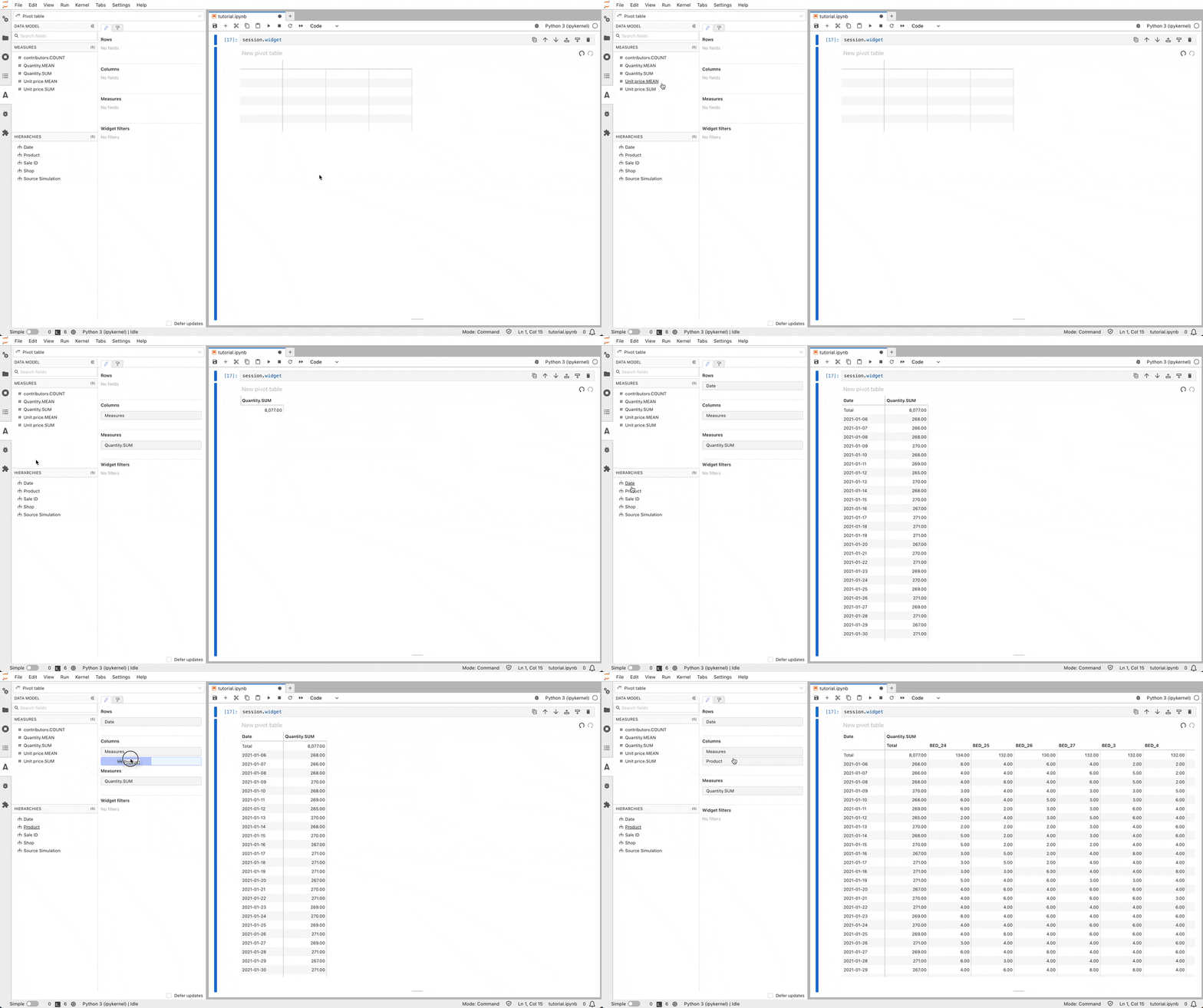
Let’s start by creating a pivot table:
* Run [`session.widget`](../../api/atoti.Session.widget#atoti.Session.widget).
* In the left panel, click on a measure such as **Quantity.SUM** to add it.
* Click on a hierarchy such as **Date** to get the quantity per date.
* Drag and drop another hierarchy such as **Product** to the **Columns** section to get the quantity sold per day and per product.
```pycon theme={"languages":{"custom":["/engine/python-sdk/6.2/languages/pycon.tmLanguage.json"]}}
>>> cube.query(
... m["Quantity.SUM"],
... levels=[l["Date"], l["Product"]],
... filter=l["Shop"] == "shop_0",
... )
Quantity.SUM
Date Product
2021-01-15 BED_24 1.00
BED_26 1.00
BED_3 1.00
BED_4 1.00
BED_46 1.00
... ...
2021-02-04 TSH_51 2.00
TSH_52 1.00
TSH_53 1.00
TSH_7 1.00
TSH_9 1.00
[125 rows x 1 columns]
```
### Interactive widget
So far we have used [`cube.query()`](../../api/atoti.Cube.query#atoti.Cube.query) which returns a pandas DataFrame but a better way to visualize multidimensional data is a pivot table.
With Atoti’s JupyterLab extension, you can create interactive widgets such as pivot tables and charts directly into your notebook.
This will create a widget and open the Atoti tab on the left with tools to manipulate the widget.
Let’s start by creating a pivot table:
* Run [`session.widget`](../../api/atoti.Session.widget#atoti.Session.widget).
* In the left panel, click on a measure such as **Quantity.SUM** to add it.
* Click on a hierarchy such as **Date** to get the quantity per date.
* Drag and drop another hierarchy such as **Product** to the **Columns** section to get the quantity sold per day and per product.
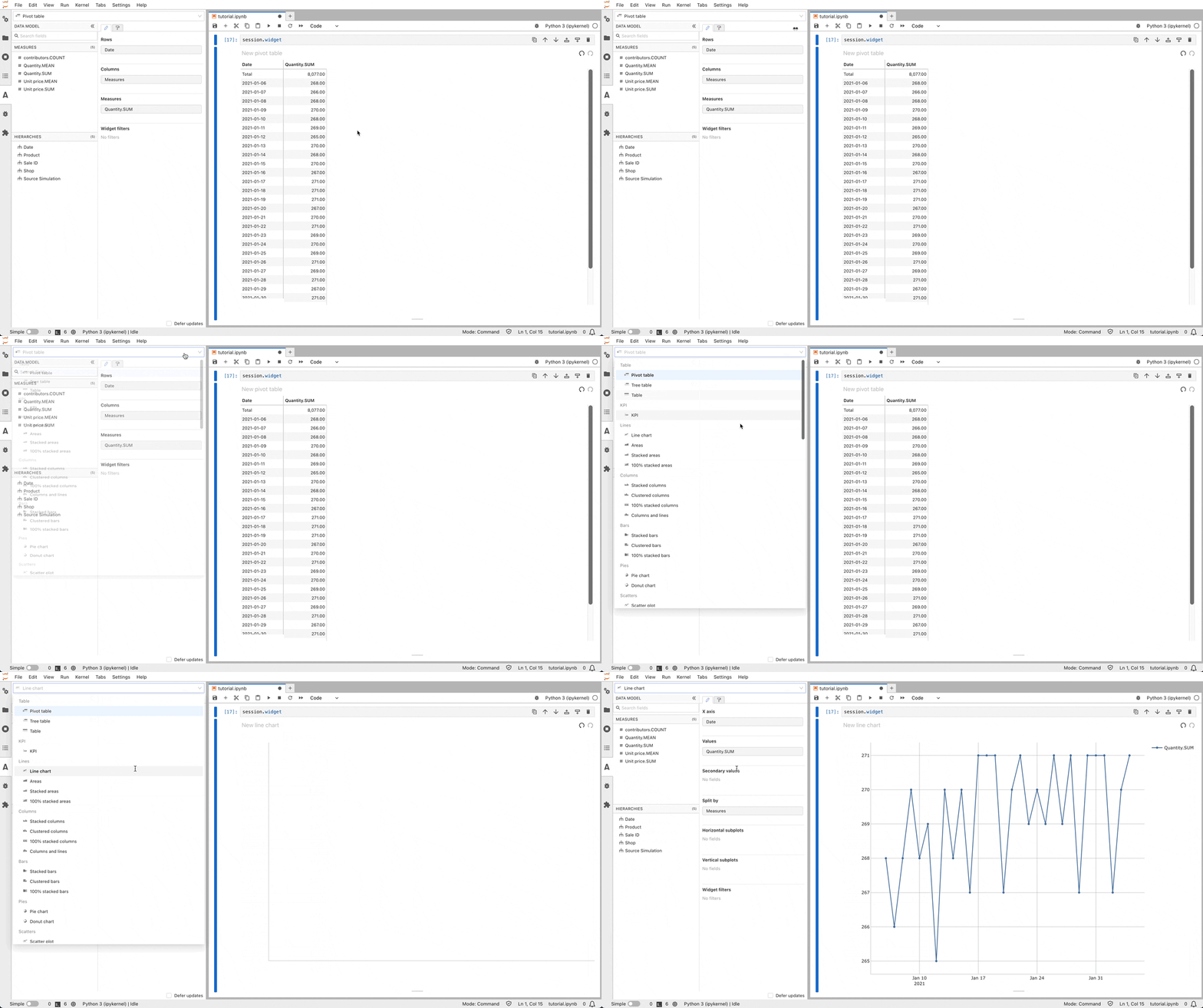
 Tables can be switched to charts.
For instance let’s switch to a line chart.
Tables can be switched to charts.
For instance let’s switch to a line chart.
 ### Drilldown and filters
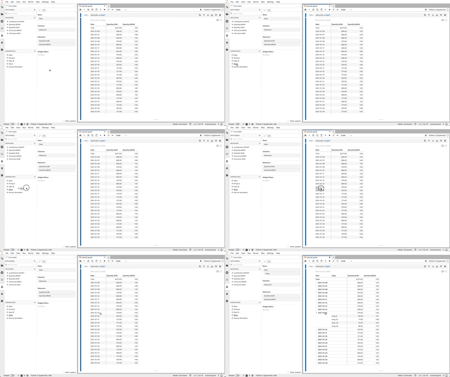
Multidimensional analysis is meant to be done from top to bottom: start by visualizing the indicators at the top level then drilldown to explain the top figures with more details.
For instance, we can visualize some measures per date then drilldown on **Shop** for a specific date, then see the products sold by a specific shop on this date.
Using the previous cube representation, this is like zooming more and more on a part of the cube.
### Drilldown and filters
Multidimensional analysis is meant to be done from top to bottom: start by visualizing the indicators at the top level then drilldown to explain the top figures with more details.
For instance, we can visualize some measures per date then drilldown on **Shop** for a specific date, then see the products sold by a specific shop on this date.
Using the previous cube representation, this is like zooming more and more on a part of the cube.

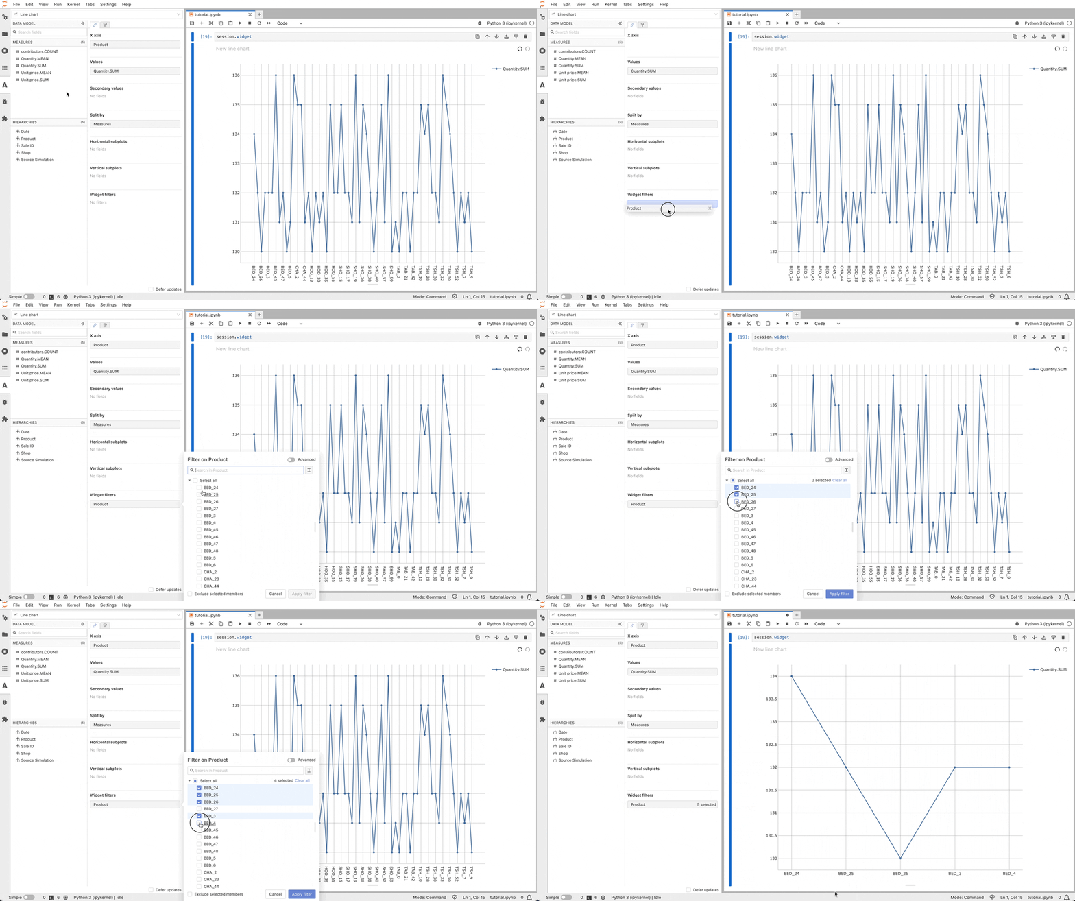
 Hierarchies can be filtered when building widgets.
Let’s apply a filter on the previous chart and only visualize the quantity for a group of selected products.
Hierarchies can be filtered when building widgets.
Let’s apply a filter on the previous chart and only visualize the quantity for a group of selected products.
 ### Dashboarding app
Being able to quickly build widgets inside a notebook without coding is nice to rapidly explore the data, iterate on your model and share some results.
However, to provide richer insights, dashboards are even better.
That’s why Atoti comes with a web app that can be accessed outside of the notebook and where widgets can be laid out to form dashboards.
The app can be accessed with this link:
```pycon theme={"languages":{"custom":["/engine/python-sdk/6.2/languages/pycon.tmLanguage.json"]}}
>>> session.link
http://localhost:9090
```
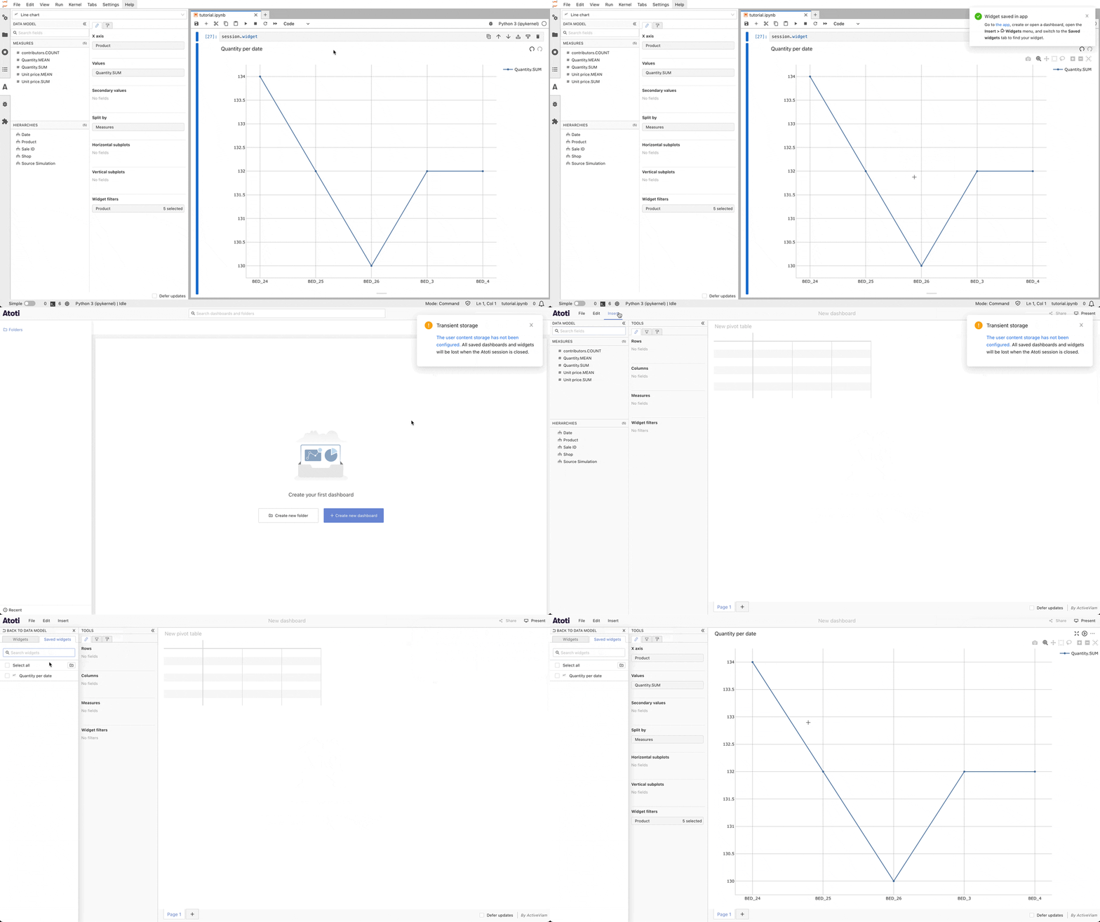
Widgets built in the notebook can be saved in the app by right clicking on them and selecting **Save widget in app**.
They will then be available in the **Saved widgets** section.
### Dashboarding app
Being able to quickly build widgets inside a notebook without coding is nice to rapidly explore the data, iterate on your model and share some results.
However, to provide richer insights, dashboards are even better.
That’s why Atoti comes with a web app that can be accessed outside of the notebook and where widgets can be laid out to form dashboards.
The app can be accessed with this link:
```pycon theme={"languages":{"custom":["/engine/python-sdk/6.2/languages/pycon.tmLanguage.json"]}}
>>> session.link
http://localhost:9090
```
Widgets built in the notebook can be saved in the app by right clicking on them and selecting **Save widget in app**.
They will then be available in the **Saved widgets** section.
 ## Enriching the cube
In the previous section, you have learned how to create a basic cube and manipulate it.
We will now enrich this cube with additional attributes and more interesting measures.
### Join
Currently, we have very limited information about our products: only the ID.
We can load a CSV containing more details into a new table:
```pycon theme={"languages":{"custom":["/engine/python-sdk/6.2/languages/pycon.tmLanguage.json"]}}
>>> products_table = session.read_csv(
... data_directory / "products.csv", keys={"Product"}, table_name="Products"
... )
```
Note that a table can have a set of keys.
These keys are the columns which make each line unique.
Here, it’s the product ID.
If you try to insert a new row with the same keys as an existing row, it will override the existing one.
```pycon theme={"languages":{"custom":["/engine/python-sdk/6.2/languages/pycon.tmLanguage.json"]}}
>>> products_table.query().set_index(list(products_table.keys)).sort_index().head()
Category Sub category Size Purchase price Color Brand
Product
BED_24 Furniture Bed Single 127.0 brown Basic
BED_25 Furniture Bed Double 252.0 black Mega
BED_26 Furniture Bed Queen 333.0 white Basic
BED_27 Furniture Bed King 375.0 blue Mega
BED_3 Furniture Bed Single 127.0 red Mega
```
This table contains the category, subcategory, size, color, purchase price and brand of the product.
Both tables have a **Product** column we can use to [`join`](../../api/atoti.Table.join#atoti.Table.join) them.
```pycon theme={"languages":{"custom":["/engine/python-sdk/6.2/languages/pycon.tmLanguage.json"]}}
>>> sales_table.join(
... products_table, sales_table["Product"] == products_table["Product"]
... )
```
Note that this is a database-like join and not a pandas-like join.
All the details from `products_table` won’t be inlined into `sales_table`.
Instead, this just declares a reference between these two tables that the cube can use to provide more analytical axes.
You can visualize the structure of the session’s tables:
```pycon theme={"languages":{"custom":["/engine/python-sdk/6.2/languages/pycon.tmLanguage.json"]}}
>>> session.tables.schema
```
```mermaid theme={"languages":{"custom":["/engine/python-sdk/6.2/languages/pycon.tmLanguage.json"]}}
erDiagram
"Sales" {
non-null String PK "Sale ID"
non-null LocalDate "Date"
non-null String "Shop"
non-null String "Product"
nullable double "Quantity"
nullable double "Unit price"
}
"Products" {
non-null String PK "Product"
non-null String "Category"
non-null String "Sub category"
non-null String "Size"
nullable double "Purchase price"
non-null String "Color"
non-null String "Brand"
}
"Sales" }o--o| "Products" : "Product == Product"
```
The new columns have been automatically added to the cube as hierarchies, in a dimension with the same name as the new table:
```pycon theme={"languages":{"custom":["/engine/python-sdk/6.2/languages/pycon.tmLanguage.json"]}}
>>> h
```
## Enriching the cube
In the previous section, you have learned how to create a basic cube and manipulate it.
We will now enrich this cube with additional attributes and more interesting measures.
### Join
Currently, we have very limited information about our products: only the ID.
We can load a CSV containing more details into a new table:
```pycon theme={"languages":{"custom":["/engine/python-sdk/6.2/languages/pycon.tmLanguage.json"]}}
>>> products_table = session.read_csv(
... data_directory / "products.csv", keys={"Product"}, table_name="Products"
... )
```
Note that a table can have a set of keys.
These keys are the columns which make each line unique.
Here, it’s the product ID.
If you try to insert a new row with the same keys as an existing row, it will override the existing one.
```pycon theme={"languages":{"custom":["/engine/python-sdk/6.2/languages/pycon.tmLanguage.json"]}}
>>> products_table.query().set_index(list(products_table.keys)).sort_index().head()
Category Sub category Size Purchase price Color Brand
Product
BED_24 Furniture Bed Single 127.0 brown Basic
BED_25 Furniture Bed Double 252.0 black Mega
BED_26 Furniture Bed Queen 333.0 white Basic
BED_27 Furniture Bed King 375.0 blue Mega
BED_3 Furniture Bed Single 127.0 red Mega
```
This table contains the category, subcategory, size, color, purchase price and brand of the product.
Both tables have a **Product** column we can use to [`join`](../../api/atoti.Table.join#atoti.Table.join) them.
```pycon theme={"languages":{"custom":["/engine/python-sdk/6.2/languages/pycon.tmLanguage.json"]}}
>>> sales_table.join(
... products_table, sales_table["Product"] == products_table["Product"]
... )
```
Note that this is a database-like join and not a pandas-like join.
All the details from `products_table` won’t be inlined into `sales_table`.
Instead, this just declares a reference between these two tables that the cube can use to provide more analytical axes.
You can visualize the structure of the session’s tables:
```pycon theme={"languages":{"custom":["/engine/python-sdk/6.2/languages/pycon.tmLanguage.json"]}}
>>> session.tables.schema
```
```mermaid theme={"languages":{"custom":["/engine/python-sdk/6.2/languages/pycon.tmLanguage.json"]}}
erDiagram
"Sales" {
non-null String PK "Sale ID"
non-null LocalDate "Date"
non-null String "Shop"
non-null String "Product"
nullable double "Quantity"
nullable double "Unit price"
}
"Products" {
non-null String PK "Product"
non-null String "Category"
non-null String "Sub category"
non-null String "Size"
nullable double "Purchase price"
non-null String "Color"
non-null String "Brand"
}
"Sales" }o--o| "Products" : "Product == Product"
```
The new columns have been automatically added to the cube as hierarchies, in a dimension with the same name as the new table:
```pycon theme={"languages":{"custom":["/engine/python-sdk/6.2/languages/pycon.tmLanguage.json"]}}
>>> h
```
- Dimensions
- Products
- Brand
- Brand
- Category
- Category
- Color
- Color
- Size
- Size
- Sub category
- Sub category
- Sales
- Date
- Date
- Product
- Product
- Sale ID
- Sale ID
- Shop
- Shop
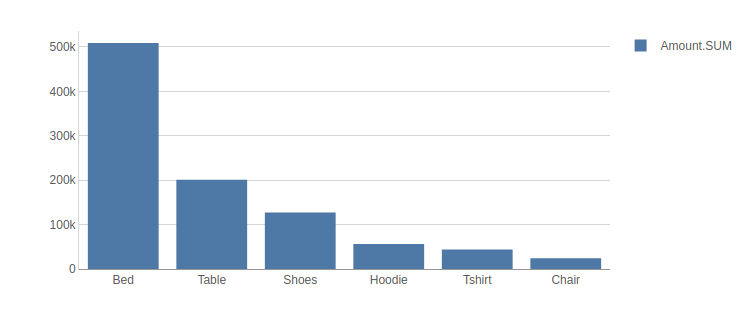
You can use them directly in a new widget.
For instance, let’s create a bar chart to visualize the mean price per subcategory of product:
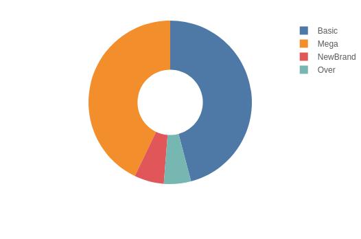
 We can also make a donut chart to see how all the sales are distributed between brands:
 Note that after the join we can add a new measure called **Purchase price.VALUE** based on the corresponding column of the joined table.
This measure represents the value of the column so it is only defined when all the keys of the joined table are expressed in the query.
```pycon theme={"languages":{"custom":["/engine/python-sdk/6.2/languages/pycon.tmLanguage.json"]}}
>>> m["Purchase price.VALUE"] = tt.agg.single_value(products_table["Purchase price"])
```
For instance we can check the purchase price per **Product**:
```pycon theme={"languages":{"custom":["/engine/python-sdk/6.2/languages/pycon.tmLanguage.json"]}}
>>> cube.query(
... m["Purchase price.VALUE"], levels=[l["Product"]]
... )
Purchase price.VALUE
Product
BED_24 127.00
BED_25 252.00
BED_26 333.00
BED_27 375.00
BED_3 127.00
... ...
TSH_52 20.00
TSH_53 21.00
TSH_7 17.00
TSH_8 18.00
TSH_9 19.00
[61 rows x 1 columns]
```
In a similar way, we can enrich the data about the shops:
```pycon theme={"languages":{"custom":["/engine/python-sdk/6.2/languages/pycon.tmLanguage.json"]}}
>>> shops_table = session.read_csv(
... data_directory / "shops.csv", keys={"Shop ID"}, table_name="Shops"
... )
>>> shops_table.query().set_index(list(shops_table.keys)).sort_index().head()
City State or region Country Shop size
Shop ID
shop_0 New York New York USA big
shop_1 Los Angeles California USA medium
shop_10 Nice Provence-Alpes-Côte d'Azur France medium
shop_11 Lyon Auvergne-Rhône-Alpes France medium
shop_12 Saint-Étienne Auvergne-Rhône-Alpes France medium
```
```pycon theme={"languages":{"custom":["/engine/python-sdk/6.2/languages/pycon.tmLanguage.json"]}}
>>> sales_table.join(shops_table, sales_table["Shop"] == shops_table["Shop ID"])
>>> session.tables.schema
```
```mermaid theme={"languages":{"custom":["/engine/python-sdk/6.2/languages/pycon.tmLanguage.json"]}}
erDiagram
"Sales" {
non-null String PK "Sale ID"
non-null LocalDate "Date"
non-null String "Shop"
non-null String "Product"
nullable double "Quantity"
nullable double "Unit price"
}
"Products" {
non-null String PK "Product"
non-null String "Category"
non-null String "Sub category"
non-null String "Size"
nullable double "Purchase price"
non-null String "Color"
non-null String "Brand"
}
"Shops" {
non-null String PK "Shop ID"
non-null String "City"
non-null String "State or region"
non-null String "Country"
non-null String "Shop size"
}
"Sales" }o--o| "Products" : "Product == Product"
"Sales" }o--o| "Shops" : "Shop == “Shop ID”"
```
### New measures
So far we have only used the default measures which are basic aggregations of the numeric columns.
We can add new custom measures to our cube.
#### Max
We’ll start with an aggregation taking the maximum price of the sales table:
```pycon theme={"languages":{"custom":["/engine/python-sdk/6.2/languages/pycon.tmLanguage.json"]}}
>>> m["Max price"] = tt.agg.max(sales_table["Unit price"])
```
This new measure is directly available:
```pycon theme={"languages":{"custom":["/engine/python-sdk/6.2/languages/pycon.tmLanguage.json"]}}
>>> cube.query(m["Max price"], include_totals=True, levels=[l["Category"]])
Max price
Category
Total 440.00
Cloth 60.00
Furniture 440.00
```
#### Fact-level operations
To compute aggregates based of data which comes directly from the columns of a table, you can pass the calculation directly to the desired aggregation function. This is more efficient than first converting the columns to measures before the aggregation.
Let’s use this to compute the total amount earned from the sale of the products, as well as the average.
```pycon theme={"languages":{"custom":["/engine/python-sdk/6.2/languages/pycon.tmLanguage.json"]}}
>>> m["Amount.SUM"] = tt.agg.sum(sales_table["Quantity"] * sales_table["Unit price"])
>>> m["Amount.MEAN"] = tt.agg.mean(
... sales_table["Quantity"] * sales_table["Unit price"],
... )
```
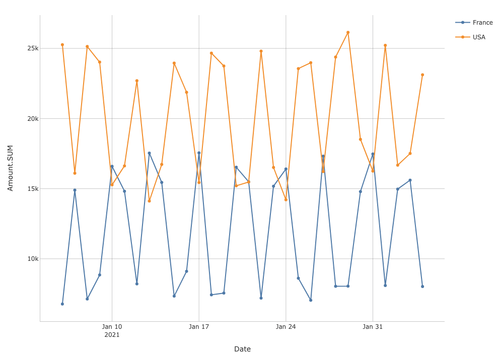
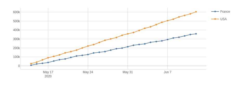
We can now plot the evolution of the sales per country over time:
Note that after the join we can add a new measure called **Purchase price.VALUE** based on the corresponding column of the joined table.
This measure represents the value of the column so it is only defined when all the keys of the joined table are expressed in the query.
```pycon theme={"languages":{"custom":["/engine/python-sdk/6.2/languages/pycon.tmLanguage.json"]}}
>>> m["Purchase price.VALUE"] = tt.agg.single_value(products_table["Purchase price"])
```
For instance we can check the purchase price per **Product**:
```pycon theme={"languages":{"custom":["/engine/python-sdk/6.2/languages/pycon.tmLanguage.json"]}}
>>> cube.query(
... m["Purchase price.VALUE"], levels=[l["Product"]]
... )
Purchase price.VALUE
Product
BED_24 127.00
BED_25 252.00
BED_26 333.00
BED_27 375.00
BED_3 127.00
... ...
TSH_52 20.00
TSH_53 21.00
TSH_7 17.00
TSH_8 18.00
TSH_9 19.00
[61 rows x 1 columns]
```
In a similar way, we can enrich the data about the shops:
```pycon theme={"languages":{"custom":["/engine/python-sdk/6.2/languages/pycon.tmLanguage.json"]}}
>>> shops_table = session.read_csv(
... data_directory / "shops.csv", keys={"Shop ID"}, table_name="Shops"
... )
>>> shops_table.query().set_index(list(shops_table.keys)).sort_index().head()
City State or region Country Shop size
Shop ID
shop_0 New York New York USA big
shop_1 Los Angeles California USA medium
shop_10 Nice Provence-Alpes-Côte d'Azur France medium
shop_11 Lyon Auvergne-Rhône-Alpes France medium
shop_12 Saint-Étienne Auvergne-Rhône-Alpes France medium
```
```pycon theme={"languages":{"custom":["/engine/python-sdk/6.2/languages/pycon.tmLanguage.json"]}}
>>> sales_table.join(shops_table, sales_table["Shop"] == shops_table["Shop ID"])
>>> session.tables.schema
```
```mermaid theme={"languages":{"custom":["/engine/python-sdk/6.2/languages/pycon.tmLanguage.json"]}}
erDiagram
"Sales" {
non-null String PK "Sale ID"
non-null LocalDate "Date"
non-null String "Shop"
non-null String "Product"
nullable double "Quantity"
nullable double "Unit price"
}
"Products" {
non-null String PK "Product"
non-null String "Category"
non-null String "Sub category"
non-null String "Size"
nullable double "Purchase price"
non-null String "Color"
non-null String "Brand"
}
"Shops" {
non-null String PK "Shop ID"
non-null String "City"
non-null String "State or region"
non-null String "Country"
non-null String "Shop size"
}
"Sales" }o--o| "Products" : "Product == Product"
"Sales" }o--o| "Shops" : "Shop == “Shop ID”"
```
### New measures
So far we have only used the default measures which are basic aggregations of the numeric columns.
We can add new custom measures to our cube.
#### Max
We’ll start with an aggregation taking the maximum price of the sales table:
```pycon theme={"languages":{"custom":["/engine/python-sdk/6.2/languages/pycon.tmLanguage.json"]}}
>>> m["Max price"] = tt.agg.max(sales_table["Unit price"])
```
This new measure is directly available:
```pycon theme={"languages":{"custom":["/engine/python-sdk/6.2/languages/pycon.tmLanguage.json"]}}
>>> cube.query(m["Max price"], include_totals=True, levels=[l["Category"]])
Max price
Category
Total 440.00
Cloth 60.00
Furniture 440.00
```
#### Fact-level operations
To compute aggregates based of data which comes directly from the columns of a table, you can pass the calculation directly to the desired aggregation function. This is more efficient than first converting the columns to measures before the aggregation.
Let’s use this to compute the total amount earned from the sale of the products, as well as the average.
```pycon theme={"languages":{"custom":["/engine/python-sdk/6.2/languages/pycon.tmLanguage.json"]}}
>>> m["Amount.SUM"] = tt.agg.sum(sales_table["Quantity"] * sales_table["Unit price"])
>>> m["Amount.MEAN"] = tt.agg.mean(
... sales_table["Quantity"] * sales_table["Unit price"],
... )
```
We can now plot the evolution of the sales per country over time:
 #### Margin
Now that the price of each product is available from the products table, we can compute the margin.
We use the [`OriginScope`](../../api/atoti.scope.OriginScope#atoti.OriginScope) to perform the multiplication of the quantity sold by the purchase price for each **Product** and then do the sum.
```pycon theme={"languages":{"custom":["/engine/python-sdk/6.2/languages/pycon.tmLanguage.json"]}}
>>> cost = tt.agg.sum(
... m["Quantity.SUM"] * tt.agg.single_value(products_table["Purchase price"]),
... scope=tt.OriginScope({l["Product"]}),
... )
```
```pycon theme={"languages":{"custom":["/engine/python-sdk/6.2/languages/pycon.tmLanguage.json"]}}
>>> m["Margin"] = m["Amount.SUM"] - cost
```
We can also define the margin rate which is the ratio of the margin by the the sold amount:
```pycon theme={"languages":{"custom":["/engine/python-sdk/6.2/languages/pycon.tmLanguage.json"]}}
>>> m["Margin rate"] = m["Margin"] / m["Amount.SUM"]
```
```pycon theme={"languages":{"custom":["/engine/python-sdk/6.2/languages/pycon.tmLanguage.json"]}}
>>> cube.query(
... m["Margin"], m["Margin rate"], levels=[l["Product"]]
... )
Margin Margin rate
Product
BED_24 3,082.00 .15
BED_25 6,336.00 .16
BED_26 8,060.00 .16
BED_27 8,580.00 .15
BED_3 3,036.00 .15
...
TSH_52 520.00 .17
TSH_53 396.00 .12
TSH_7 393.00 .15
TSH_8 264.00 .10
TSH_9 390.00 .14
[61 rows x 2 columns]
```
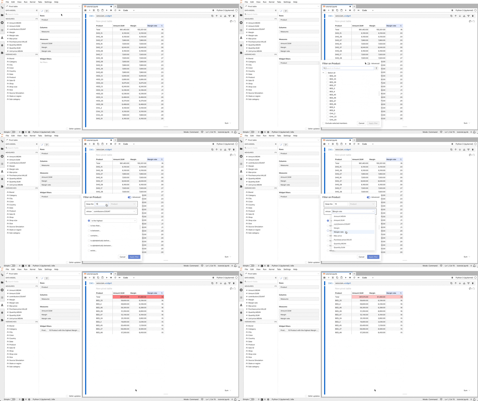
Let’s use this margin rate to do a *Top 10* filter to see the products with the best rate.
Note that you don’t need to put the rate measure and the product level in the pivot table to apply the filter.
#### Margin
Now that the price of each product is available from the products table, we can compute the margin.
We use the [`OriginScope`](../../api/atoti.scope.OriginScope#atoti.OriginScope) to perform the multiplication of the quantity sold by the purchase price for each **Product** and then do the sum.
```pycon theme={"languages":{"custom":["/engine/python-sdk/6.2/languages/pycon.tmLanguage.json"]}}
>>> cost = tt.agg.sum(
... m["Quantity.SUM"] * tt.agg.single_value(products_table["Purchase price"]),
... scope=tt.OriginScope({l["Product"]}),
... )
```
```pycon theme={"languages":{"custom":["/engine/python-sdk/6.2/languages/pycon.tmLanguage.json"]}}
>>> m["Margin"] = m["Amount.SUM"] - cost
```
We can also define the margin rate which is the ratio of the margin by the the sold amount:
```pycon theme={"languages":{"custom":["/engine/python-sdk/6.2/languages/pycon.tmLanguage.json"]}}
>>> m["Margin rate"] = m["Margin"] / m["Amount.SUM"]
```
```pycon theme={"languages":{"custom":["/engine/python-sdk/6.2/languages/pycon.tmLanguage.json"]}}
>>> cube.query(
... m["Margin"], m["Margin rate"], levels=[l["Product"]]
... )
Margin Margin rate
Product
BED_24 3,082.00 .15
BED_25 6,336.00 .16
BED_26 8,060.00 .16
BED_27 8,580.00 .15
BED_3 3,036.00 .15
...
TSH_52 520.00 .17
TSH_53 396.00 .12
TSH_7 393.00 .15
TSH_8 264.00 .10
TSH_9 390.00 .14
[61 rows x 2 columns]
```
Let’s use this margin rate to do a *Top 10* filter to see the products with the best rate.
Note that you don’t need to put the rate measure and the product level in the pivot table to apply the filter.
 #### Cumulative sum over time
A cumulative sum is the partial sum of the data up to the current value.
For instance, a cumulative sum over time can be used to show how some measure changes over time.
```pycon theme={"languages":{"custom":["/engine/python-sdk/6.2/languages/pycon.tmLanguage.json"]}}
>>> m["Cumulative amount"] = tt.agg.sum(
... m["Amount.SUM"],
... scope=tt.CumulativeScope(l["Date"]),
... )
```
#### Cumulative sum over time
A cumulative sum is the partial sum of the data up to the current value.
For instance, a cumulative sum over time can be used to show how some measure changes over time.
```pycon theme={"languages":{"custom":["/engine/python-sdk/6.2/languages/pycon.tmLanguage.json"]}}
>>> m["Cumulative amount"] = tt.agg.sum(
... m["Amount.SUM"],
... scope=tt.CumulativeScope(l["Date"]),
... )
```
 #### Average per shop
Aggregations can also be combined.
For instance, we can sum inside a **Shop**: then take the average of this to see how much a table sales on average:
```pycon theme={"languages":{"custom":["/engine/python-sdk/6.2/languages/pycon.tmLanguage.json"]}}
>>> m["Average amount per shop"] = tt.agg.mean(
... m["Amount.SUM"],
... scope=tt.OriginScope({l["Shop"]}),
... )
```
```pycon theme={"languages":{"custom":["/engine/python-sdk/6.2/languages/pycon.tmLanguage.json"]}}
>>> cube.query(
... m["Average amount per shop"],
... include_totals=True,
... levels=[l["Sub category"]],
... )
Average amount per shop
Sub category
Total 24,036.58
Bed 12,728.88
Chair 601.50
Hoodie 1,403.20
Shoes 3,184.50
T-shirt 1,095.00
Table 5,023.50
```
### Multilevel hierarchies
So far, all our hierarchies only had one level but it’s best to regroup attributes with a parent-child relationship in the same hierarchy.
For example, we can group the **Category**, **SubCategory** and **Product ID** levels into a **Product** hierarchy:
```pycon theme={"languages":{"custom":["/engine/python-sdk/6.2/languages/pycon.tmLanguage.json"]}}
>>> h["Product"] = [l["Category"], l["Sub category"], l["Product"]]
```
And let’s remove the old hierarchies:
```pycon theme={"languages":{"custom":["/engine/python-sdk/6.2/languages/pycon.tmLanguage.json"]}}
>>> del h["Category"]
>>> del h["Sub category"]
```
```pycon theme={"languages":{"custom":["/engine/python-sdk/6.2/languages/pycon.tmLanguage.json"]}}
>>> h
```
#### Average per shop
Aggregations can also be combined.
For instance, we can sum inside a **Shop**: then take the average of this to see how much a table sales on average:
```pycon theme={"languages":{"custom":["/engine/python-sdk/6.2/languages/pycon.tmLanguage.json"]}}
>>> m["Average amount per shop"] = tt.agg.mean(
... m["Amount.SUM"],
... scope=tt.OriginScope({l["Shop"]}),
... )
```
```pycon theme={"languages":{"custom":["/engine/python-sdk/6.2/languages/pycon.tmLanguage.json"]}}
>>> cube.query(
... m["Average amount per shop"],
... include_totals=True,
... levels=[l["Sub category"]],
... )
Average amount per shop
Sub category
Total 24,036.58
Bed 12,728.88
Chair 601.50
Hoodie 1,403.20
Shoes 3,184.50
T-shirt 1,095.00
Table 5,023.50
```
### Multilevel hierarchies
So far, all our hierarchies only had one level but it’s best to regroup attributes with a parent-child relationship in the same hierarchy.
For example, we can group the **Category**, **SubCategory** and **Product ID** levels into a **Product** hierarchy:
```pycon theme={"languages":{"custom":["/engine/python-sdk/6.2/languages/pycon.tmLanguage.json"]}}
>>> h["Product"] = [l["Category"], l["Sub category"], l["Product"]]
```
And let’s remove the old hierarchies:
```pycon theme={"languages":{"custom":["/engine/python-sdk/6.2/languages/pycon.tmLanguage.json"]}}
>>> del h["Category"]
>>> del h["Sub category"]
```
```pycon theme={"languages":{"custom":["/engine/python-sdk/6.2/languages/pycon.tmLanguage.json"]}}
>>> h
```
- Dimensions
- Products
- Brand
- Brand
- Color
- Color
- Product
- Category
- Sub category
- Product
- Size
- Size
- Sales
- Date
- Date
- Product
- Product
- Sale ID
- Sale ID
- Shop
- Shop
- Shops
- City
- City
- Country
- Country
- Shop size
- Shop size
- State or region
- State or region
We can also do it with **City**, **State or Region** and **Country** to build a **Geography** hierarchy.
Note that instead of using existing levels you can also define a hierarchy with the columns of the table the levels will be based on:
```pycon theme={"languages":{"custom":["/engine/python-sdk/6.2/languages/pycon.tmLanguage.json"]}}
>>> h["Geography"] = [
... shops_table["Country"],
... shops_table["State or region"],
... shops_table["City"],
... ]
>>> del h["Country"]
>>> del h["State or region"]
>>> del h["City"]
```
As we are restructuring the hierarchies, let’s use this opportunity to also change the dimensions.
A dimension regroups hierarchies of the same concept.
We can move the new **Geography** hierarchy to its own dimension:
```pycon theme={"languages":{"custom":["/engine/python-sdk/6.2/languages/pycon.tmLanguage.json"]}}
>>> h["Geography"].dimension_name = "Location"
>>> h
```
- Dimensions
- Location
- Geography
- Country
- State or region
- City
- Products
- Brand
- Brand
- Color
- Color
- Product
- Category
- Sub category
- Product
- Size
- Size
- Sales
- Date
- Date
- Product
- Product
- Sale ID
- Sale ID
- Shop
- Shop
- Shops
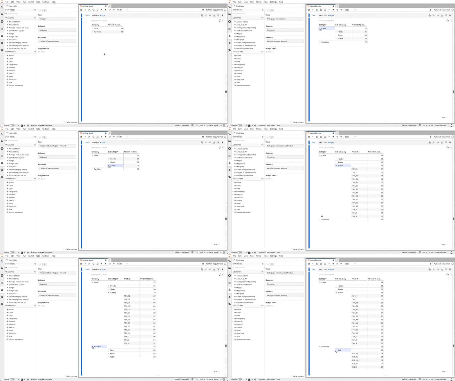
With that, we can define new measures taking advantage of the multilevel structure.
For instance, we can create a measure indicating how much a product contributes to its subcategory:
```pycon theme={"languages":{"custom":["/engine/python-sdk/6.2/languages/pycon.tmLanguage.json"]}}
>>> m["Parent category amount"] = tt.parent_value(
... m["Amount.SUM"],
... degrees={h["Products", "Product"]: 1},
... )
```
```pycon theme={"languages":{"custom":["/engine/python-sdk/6.2/languages/pycon.tmLanguage.json"]}}
>>> m["Percent of parent amount"] = m["Amount.SUM"] / m["Parent category amount"]
```
 ## Polishing the cube
### Deleting or hiding measures
Some measures have been automatically created from numeric columns but are not useful.
For instance, **Unit Price.SUM** does not really make sense as we never want to sum the unit prices.
We can delete it:
```pycon theme={"languages":{"custom":["/engine/python-sdk/6.2/languages/pycon.tmLanguage.json"]}}
>>> del m["Unit price.SUM"]
```
Other measures have been used while building the project only as intermediary steps but are not useful to the end users in the app.
We can hide them from the UI (they will remain accessible in Python):
```pycon theme={"languages":{"custom":["/engine/python-sdk/6.2/languages/pycon.tmLanguage.json"]}}
>>> m["Parent category amount"].visible = False
```
### Measure folders
Measures can be rearranged into folders.
```pycon theme={"languages":{"custom":["/engine/python-sdk/6.2/languages/pycon.tmLanguage.json"]}}
>>> for measure in [
... m["Amount.MEAN"],
... m["Amount.SUM"],
... m["Average amount per shop"],
... m["Cumulative amount"],
... m["Percent of parent amount"],
... ]:
... measure.folder = "Amount"
```
```pycon theme={"languages":{"custom":["/engine/python-sdk/6.2/languages/pycon.tmLanguage.json"]}}
>>> m
```
## Polishing the cube
### Deleting or hiding measures
Some measures have been automatically created from numeric columns but are not useful.
For instance, **Unit Price.SUM** does not really make sense as we never want to sum the unit prices.
We can delete it:
```pycon theme={"languages":{"custom":["/engine/python-sdk/6.2/languages/pycon.tmLanguage.json"]}}
>>> del m["Unit price.SUM"]
```
Other measures have been used while building the project only as intermediary steps but are not useful to the end users in the app.
We can hide them from the UI (they will remain accessible in Python):
```pycon theme={"languages":{"custom":["/engine/python-sdk/6.2/languages/pycon.tmLanguage.json"]}}
>>> m["Parent category amount"].visible = False
```
### Measure folders
Measures can be rearranged into folders.
```pycon theme={"languages":{"custom":["/engine/python-sdk/6.2/languages/pycon.tmLanguage.json"]}}
>>> for measure in [
... m["Amount.MEAN"],
... m["Amount.SUM"],
... m["Average amount per shop"],
... m["Cumulative amount"],
... m["Percent of parent amount"],
... ]:
... measure.folder = "Amount"
```
```pycon theme={"languages":{"custom":["/engine/python-sdk/6.2/languages/pycon.tmLanguage.json"]}}
>>> m
```
- Measures
- 📁 Amount
- Amount.MEAN
- formatter: DOUBLE\[#,###.00]
- Amount.SUM
- formatter: DOUBLE\[#,###.00]
- Average amount per shop
- formatter: DOUBLE\[#,###.00]
- Cumulative amount
- formatter: DOUBLE\[#,###.00]
- Percent of parent amount
- formatter: DOUBLE\[#,###.00]
- Margin
- formatter: DOUBLE\[#,###.00]
- Margin rate
- formatter: DOUBLE\[#,###.00]
- Max price
- formatter: DOUBLE\[#,###.00]
- Purchase price.VALUE
- formatter: DOUBLE\[#,###.00]
- Quantity.MEAN
- formatter: DOUBLE\[#,###.00]
- Quantity.SUM
- formatter: DOUBLE\[#,###.00]
- Unit price.MEAN
- formatter: DOUBLE\[#,###.00]
- contributors.COUNT
### Measure formatters
Some measures can be formatted for a nicer display.
Classic examples of this is changing the number of decimals or adding a percent or a currency symbol.
Let’s do this for our percent of parent amount and margin rate:
#### Before
```pycon theme={"languages":{"custom":["/engine/python-sdk/6.2/languages/pycon.tmLanguage.json"]}}
>>> cube.query(m["Percent of parent amount"], m["Margin rate"], levels=[l["Category"]])
Percent of parent amount Margin rate
Category
Cloth .24 .23
Furniture .76 .13
```
```pycon theme={"languages":{"custom":["/engine/python-sdk/6.2/languages/pycon.tmLanguage.json"]}}
>>> m["Percent of parent amount"].formatter = "DOUBLE[0.00%]"
>>> m["Margin rate"].formatter = "DOUBLE[0.00%]"
```
#### After
```pycon theme={"languages":{"custom":["/engine/python-sdk/6.2/languages/pycon.tmLanguage.json"]}}
>>> cube.query(m["Percent of parent amount"], m["Margin rate"], levels=[l["Category"]])
Percent of parent amount Margin rate
Category
Cloth 23.64% 22.56%
Furniture 76.36% 13.49%
```
## Simulations
Simulations are a way to compare several scenarios and do what-if analysis.
This helps understanding how changing the source data or a piece of the model impact the key indicators.
In Atoti, the data model is made of measures chained together.
A simulation can be seen as changing one part of the model, either its source data or one of its measure definitions, and then evaluating how it impacts the following measures.
### Source simulation
Let’s start by changing the source.
With pandas or Spark, if you want to compare two results for a different versions of the entry dataset you have to reapply all the transformations to your dataset.
With Atoti, you only have to provide the new data and all the measures will be automatically available for both versions of the data.
We will create a new scenario using pandas to modify the original dataset.
```pycon theme={"languages":{"custom":["/engine/python-sdk/6.2/languages/pycon.tmLanguage.json"]}}
>>> import pandas as pd
```
For instance, we can simulate what would happen if we had managed to purchase some products at a cheaper price.
```pycon theme={"languages":{"custom":["/engine/python-sdk/6.2/languages/pycon.tmLanguage.json"]}}
>>> products_df = pd.read_csv(data_directory / "products.csv")
>>> products_df.head()
Product Category Sub category Size Purchase price Color Brand
0 TAB_0 Furniture Table 1m80 190.0 black Basic
1 TAB_1 Furniture Table 2m40 280.0 white Mega
2 CHA_2 Furniture Chair NaN 48.0 blue Basic
3 BED_3 Furniture Bed Single 127.0 red Mega
4 BED_4 Furniture Bed Double 252.0 brown Basic
```
```pycon theme={"languages":{"custom":["/engine/python-sdk/6.2/languages/pycon.tmLanguage.json"]}}
>>> better_prices = {
... "TAB_0": 180.0,
... "TAB_1": 250.0,
... "CHA_2": 40.0,
... "BED_3": 110.0,
... "BED_4": 210.0,
... }
```
```pycon theme={"languages":{"custom":["/engine/python-sdk/6.2/languages/pycon.tmLanguage.json"]}}
>>> for product, purchase_price in better_prices.items():
... products_df.loc[products_df["Product"] == product, "Purchase price"] = (
... purchase_price
... )
>>> products_df.head()
Product Category Sub category Size Purchase price Color Brand
0 TAB_0 Furniture Table 1m80 180.0 black Basic
1 TAB_1 Furniture Table 2m40 250.0 white Mega
2 CHA_2 Furniture Chair NaN 40.0 blue Basic
3 BED_3 Furniture Bed Single 110.0 red Mega
4 BED_4 Furniture Bed Double 210.0 brown Basic
```
We can now load this new dataframe into a new scenarios of the products table.
```pycon theme={"languages":{"custom":["/engine/python-sdk/6.2/languages/pycon.tmLanguage.json"]}}
>>> products_table.scenarios["Cheaper purchase prices"].load(products_df)
```
The session now has two scenarios and the only differences between them are the lines corresponding to the products with better prices, everything else is shared between the scenarios and has not been duplicated: source scenarios in Atoti are memory-efficient.
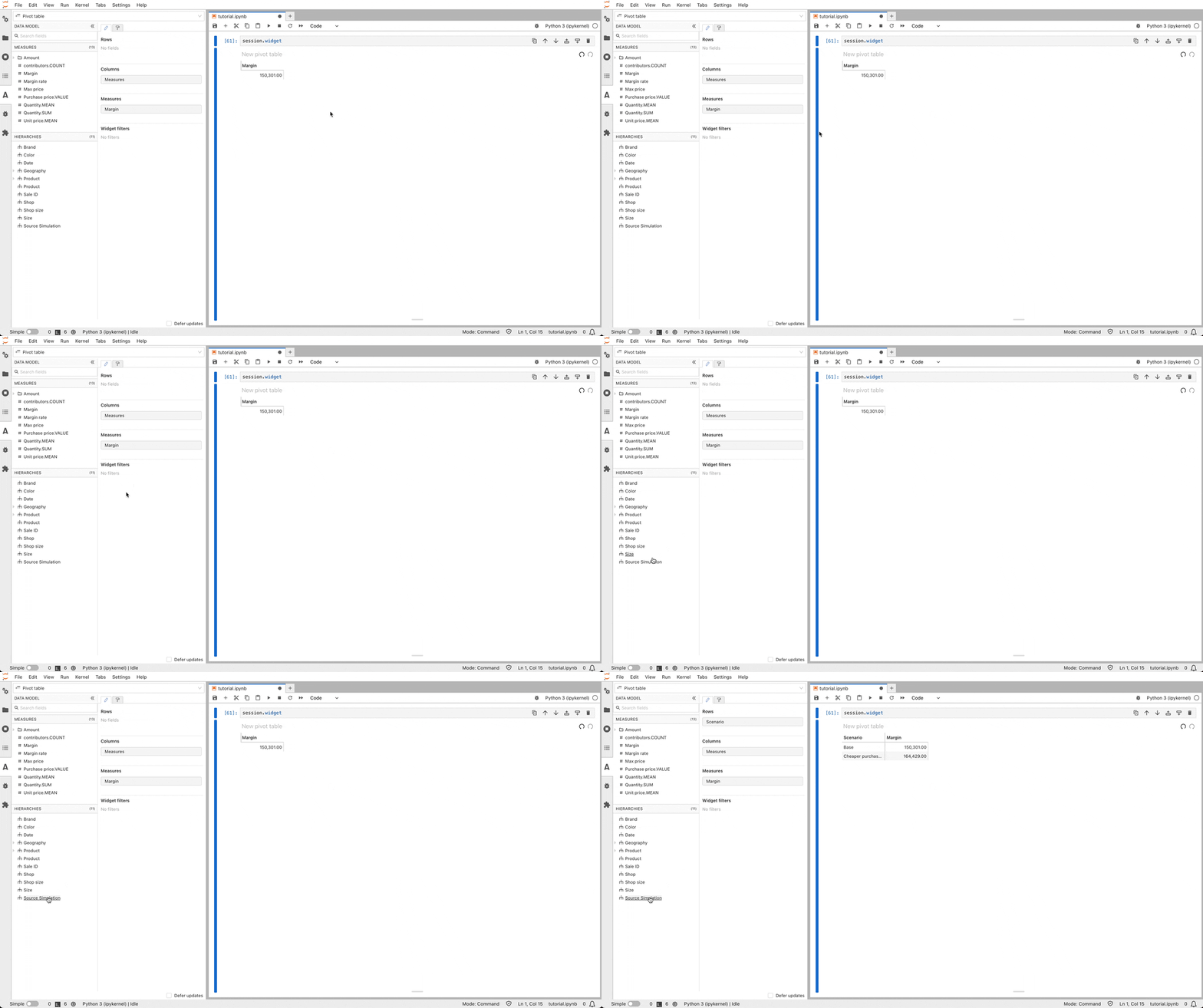
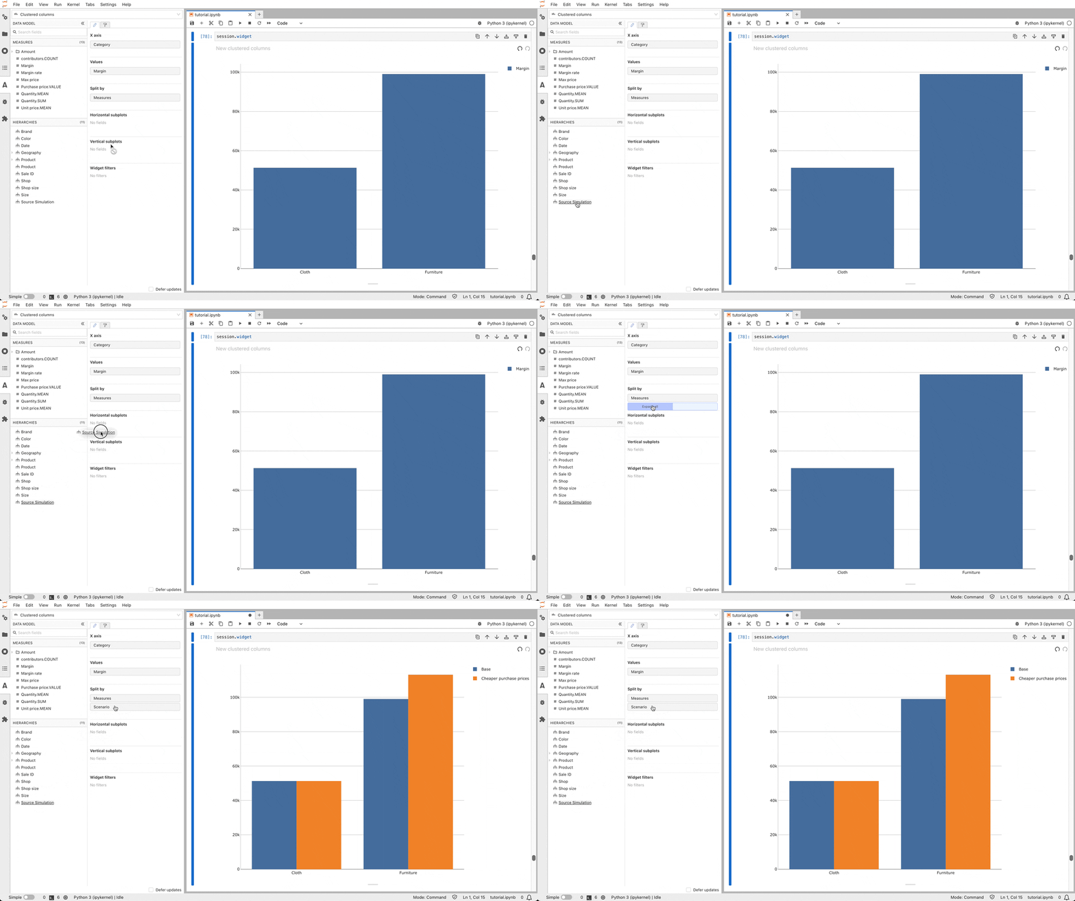
 Using the **Source Simulation** hierarchy we can display the margin of the scenario and compare it to the base case.
 Note that all the existing measures are immediately available on the new data.
For instance, the margin rate still exists, and we can see that in this scenario we would have a better margin for the Furniture products.
Note that all the existing measures are immediately available on the new data.
For instance, the margin rate still exists, and we can see that in this scenario we would have a better margin for the Furniture products.
 ### Parameter simulations
The other simulation technique is to create a parameter measure whose value can be changed for some coordinates.
When creating the simulation, you can choose at which granularity the modification applies.
For instance we can create a parameter measure whose value will change depending on the country.
Doing that, we can answer questions such as “What happens if there is a crisis in France and we sell 20% less?”
```pycon theme={"languages":{"custom":["/engine/python-sdk/6.2/languages/pycon.tmLanguage.json"]}}
>>> country_simulation = cube.create_parameter_simulation(
... "Country Simulation",
... levels=[l["Country"]],
... measures={"Country parameter": 1.0},
... )
```
This has created a measure named **Country parameter** and added it to the cube. For now, its value is `1` everywhere, but using the `country_simulation` we can change that.
By adding values in the table you can change the value of the parameter measure depending on the levels used in the simulation and the scenario.
```pycon theme={"languages":{"custom":["/engine/python-sdk/6.2/languages/pycon.tmLanguage.json"]}}
>>> country_simulation += ("France Crisis", "France", 0.80)
>>> country_simulation.head()
Country parameter
Scenario Country
France Crisis France 0.8
```
Let’s replace the existing **Quantity.SUM** and **Amount.SUM** measures with new ones using the parameter measure from the simulation.
```pycon theme={"languages":{"custom":["/engine/python-sdk/6.2/languages/pycon.tmLanguage.json"]}}
>>> m["Quantity.SUM"] = tt.agg.sum(
... tt.agg.sum(sales_table["Quantity"]) * m["Country parameter"],
... scope=tt.OriginScope({l["Country"]}),
... )
>>> m["Amount.SUM"] = tt.agg.sum(
... tt.agg.sum(sales_table["Unit price"] * sales_table["Quantity"])
... * m["Country parameter"],
... scope=tt.OriginScope({l["Country"]}),
... )
```
We can query the cube using the new **Country Simulation** level to compare the quantity and amount between the base case and our new scenario:
```pycon theme={"languages":{"custom":["/engine/python-sdk/6.2/languages/pycon.tmLanguage.json"]}}
>>> cube.query(
... m["Quantity.SUM"],
... m["Amount.SUM"],
... include_totals=True,
... levels=[l["Country Simulation"], l["Country"]],
... )
Quantity.SUM Amount.SUM
Country Simulation Country
Base 8,077.00 961,463.00
France 3,027.00 358,042.00
USA 5,050.00 603,421.00
France Crisis 7,471.60 889,854.60
France 2,421.60 286,433.60
USA 5,050.00 603,421.00
```
Here for example, as the amount has been modified, the measures depending on it such as the cumulative amount are also impacted:
```pycon theme={"languages":{"custom":["/engine/python-sdk/6.2/languages/pycon.tmLanguage.json"]}}
>>> cube.query(m["Cumulative amount"], levels=[l["Country Simulation"], l["Country"]])
Cumulative amount
Country Simulation Country
Base France 358,042.00
USA 603,421.00
France Crisis France 286,433.60
USA 603,421.00
```
Let’s try adding a different scenario:
```pycon theme={"languages":{"custom":["/engine/python-sdk/6.2/languages/pycon.tmLanguage.json"]}}
>>> country_simulation += ("US boost", "USA", 1.15)
```
```pycon theme={"languages":{"custom":["/engine/python-sdk/6.2/languages/pycon.tmLanguage.json"]}}
>>> cube.query(m["Quantity.SUM"], levels=[l["Country Simulation"], l["Country"]])
Quantity.SUM
Country Simulation Country
Base France 3,027.00
USA 5,050.00
France Crisis France 2,421.60
USA 5,050.00
US boost France 3,027.00
USA 5,807.50
```
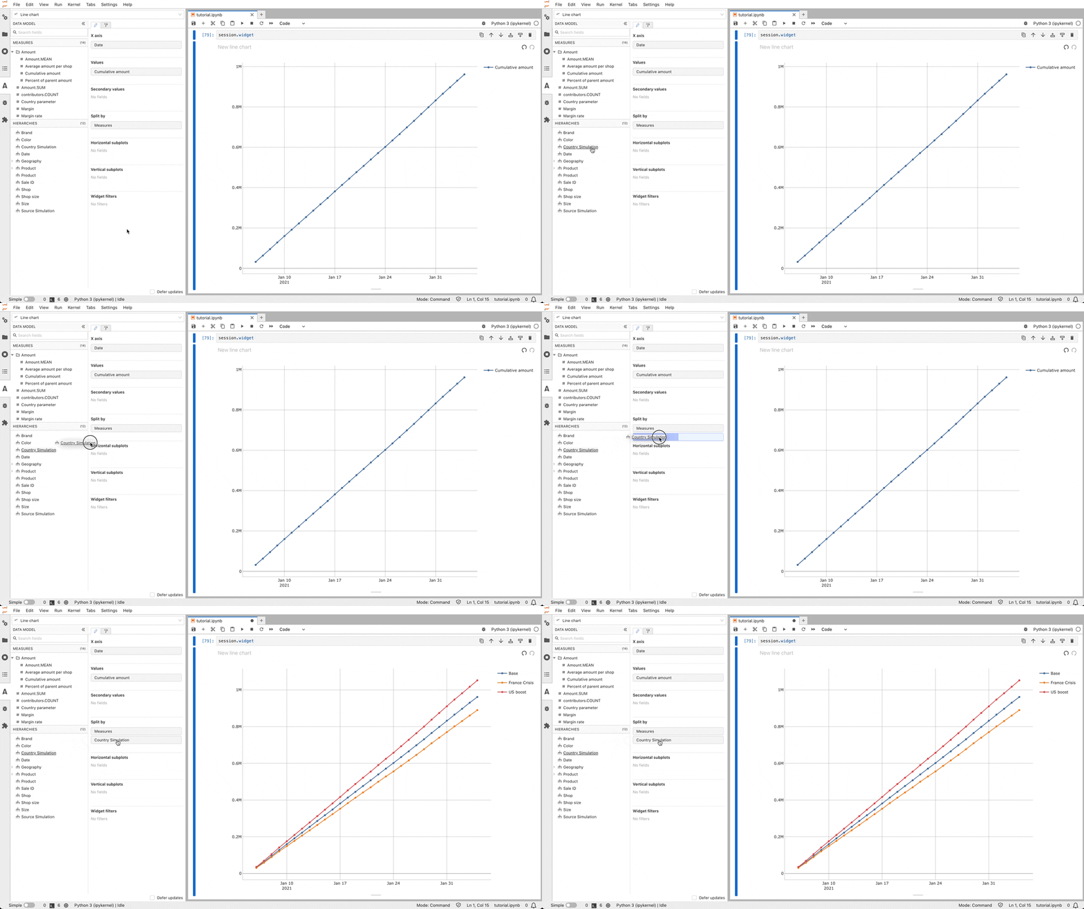
The two scenarios can be visualized in the same widget:
### Parameter simulations
The other simulation technique is to create a parameter measure whose value can be changed for some coordinates.
When creating the simulation, you can choose at which granularity the modification applies.
For instance we can create a parameter measure whose value will change depending on the country.
Doing that, we can answer questions such as “What happens if there is a crisis in France and we sell 20% less?”
```pycon theme={"languages":{"custom":["/engine/python-sdk/6.2/languages/pycon.tmLanguage.json"]}}
>>> country_simulation = cube.create_parameter_simulation(
... "Country Simulation",
... levels=[l["Country"]],
... measures={"Country parameter": 1.0},
... )
```
This has created a measure named **Country parameter** and added it to the cube. For now, its value is `1` everywhere, but using the `country_simulation` we can change that.
By adding values in the table you can change the value of the parameter measure depending on the levels used in the simulation and the scenario.
```pycon theme={"languages":{"custom":["/engine/python-sdk/6.2/languages/pycon.tmLanguage.json"]}}
>>> country_simulation += ("France Crisis", "France", 0.80)
>>> country_simulation.head()
Country parameter
Scenario Country
France Crisis France 0.8
```
Let’s replace the existing **Quantity.SUM** and **Amount.SUM** measures with new ones using the parameter measure from the simulation.
```pycon theme={"languages":{"custom":["/engine/python-sdk/6.2/languages/pycon.tmLanguage.json"]}}
>>> m["Quantity.SUM"] = tt.agg.sum(
... tt.agg.sum(sales_table["Quantity"]) * m["Country parameter"],
... scope=tt.OriginScope({l["Country"]}),
... )
>>> m["Amount.SUM"] = tt.agg.sum(
... tt.agg.sum(sales_table["Unit price"] * sales_table["Quantity"])
... * m["Country parameter"],
... scope=tt.OriginScope({l["Country"]}),
... )
```
We can query the cube using the new **Country Simulation** level to compare the quantity and amount between the base case and our new scenario:
```pycon theme={"languages":{"custom":["/engine/python-sdk/6.2/languages/pycon.tmLanguage.json"]}}
>>> cube.query(
... m["Quantity.SUM"],
... m["Amount.SUM"],
... include_totals=True,
... levels=[l["Country Simulation"], l["Country"]],
... )
Quantity.SUM Amount.SUM
Country Simulation Country
Base 8,077.00 961,463.00
France 3,027.00 358,042.00
USA 5,050.00 603,421.00
France Crisis 7,471.60 889,854.60
France 2,421.60 286,433.60
USA 5,050.00 603,421.00
```
Here for example, as the amount has been modified, the measures depending on it such as the cumulative amount are also impacted:
```pycon theme={"languages":{"custom":["/engine/python-sdk/6.2/languages/pycon.tmLanguage.json"]}}
>>> cube.query(m["Cumulative amount"], levels=[l["Country Simulation"], l["Country"]])
Cumulative amount
Country Simulation Country
Base France 358,042.00
USA 603,421.00
France Crisis France 286,433.60
USA 603,421.00
```
Let’s try adding a different scenario:
```pycon theme={"languages":{"custom":["/engine/python-sdk/6.2/languages/pycon.tmLanguage.json"]}}
>>> country_simulation += ("US boost", "USA", 1.15)
```
```pycon theme={"languages":{"custom":["/engine/python-sdk/6.2/languages/pycon.tmLanguage.json"]}}
>>> cube.query(m["Quantity.SUM"], levels=[l["Country Simulation"], l["Country"]])
Quantity.SUM
Country Simulation Country
Base France 3,027.00
USA 5,050.00
France Crisis France 2,421.60
USA 5,050.00
US boost France 3,027.00
USA 5,807.50
```
The two scenarios can be visualized in the same widget:
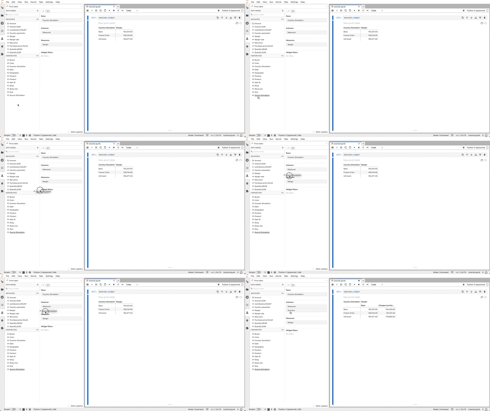
 Finally, we can even combine the different simulations (the source one and the measure one) to create a matrix of scenarios:
 ## Going further
You’ve learned all the basics to build a project with Atoti, from the concept of multidimensional analysis to powerful simulations.
We now encourage you to try the library with your own data.
You can also start to learn more advanced features such as [`SessionConfig`](../../api/atoti.config.SessionConfig#atoti.SessionConfig), [`endpoint()`](../../api/atoti.Session.endpoint#atoti.Session.endpoint), and [`array`](../../api/atoti.array#module-atoti.array).
## Going further
You’ve learned all the basics to build a project with Atoti, from the concept of multidimensional analysis to powerful simulations.
We now encourage you to try the library with your own data.
You can also start to learn more advanced features such as [`SessionConfig`](../../api/atoti.config.SessionConfig#atoti.SessionConfig), [`endpoint()`](../../api/atoti.Session.endpoint#atoti.Session.endpoint), and [`array`](../../api/atoti.array#module-atoti.array).